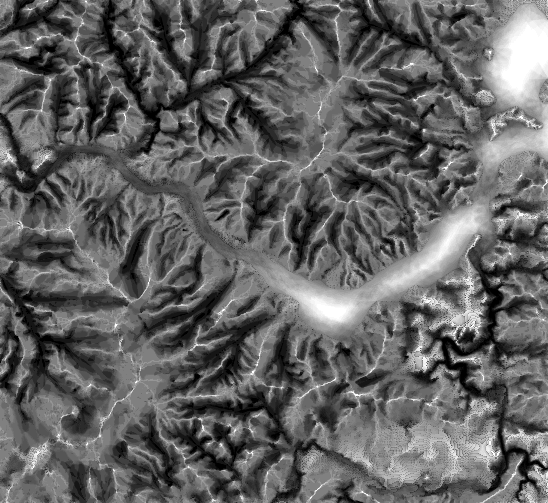
Draining Lake Mead: Making Beautiful Maps with Rayshader
(See the bottom of the page for a description on how I generated the above figure–and read the rest of the article to see how to use rayshader and R to make beautiful maps yourself. I’m also available to create custom maps–contact me for a quote.)
My most memorable experience with cartography occurred in Rome last October where I found myself briskly walking down an amazing map-covered hallway in the Vatican museum, towards the Sistine Chapel, looking around and thinking to myself “I sure hope there’s a way to get back here.” My wife and I bought tickets to have breakfast at the Vatican–which was really a roundabout way to see the Sistine Chapel before the crowds arrived. We had quickly finished our (very rushed, very un-Italian) breakfast, and started towards the Sistine Chapel as soon as we were allowed. On our way, we entered a 350 foot-long hallway that was absolutely covered in beautiful maps, illustrating the entirety of the Italian peninsula in forty large-scale frescos. I slowed down my pace, but there was no time to waste–we bought these tickets for a reason. But I wanted to get back.
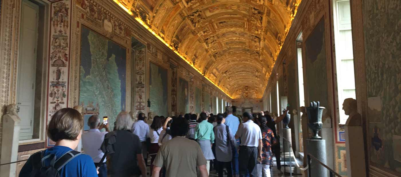
And I did get back to what I later found out was (aptly named) the Gallery of Maps. They don’t make it easy–you can’t go backwards through the museum, and I had to ask a security guard for permission to loop back around. But seeing the Italian landscape represented like it was the first few pages of a fantasy novel was incredible. The maps themselves were detailed and beautifully illustrated, and it was a nice example of combining cartography as art. The mountains, sea, hills of Italy, painted and beautifully illustrated–It got me thinking: what if there was an R package that could do just that?
… I kid, of course–no real-life human would take in the grandeur of the Vatican and think: “THIS HAS INSPIRED ME… TO DEVELOP SOFTWARE 🤖.” But there’s something about a beautiful, detailed map that’s a joy to behold. And I have developed an R package that easily produces beautiful stylized maps, and I’m going to show you how to do it as well.
rayshader can produce with the new features added in the latest version (spherical texture mapping, lambertian reflectance, ambient occlusion, water detection).
The initial version of rayshader was simple–it took a elevation matrix, traced lines towards a light source at each point, and subtracted light from that point if it ran into the ground in the process. It had the bare minimum number of features you could have to call it a raytracer: rays and, well, traces. But once it was working and making pretty pictures, I whipped up a blog post and released it to the public. And the response immediately drove the development of rayshader to a very cool place.
Ask the internet how to do something and you’re likely to get a bunch of digital shrugs and maybe—if you’re lucky—a passive aggressive link to a Wikipedia page. Tell the internet you’ve done something—and they’ll tell you exactly what you can do to improve it. By telling you everything (they thought 🤔) you did wrong. There was some great initial positive feedback, but also a bunch of notes from a few people describing what they thought was missing. One person was aghast that my raytracer didn’t have Lambertian reflectance, which is the technical term for the fact that surfaces pointing towards the light are brighter than those askew. Reasonable suggestion, I thought, so–I’ll implement it.
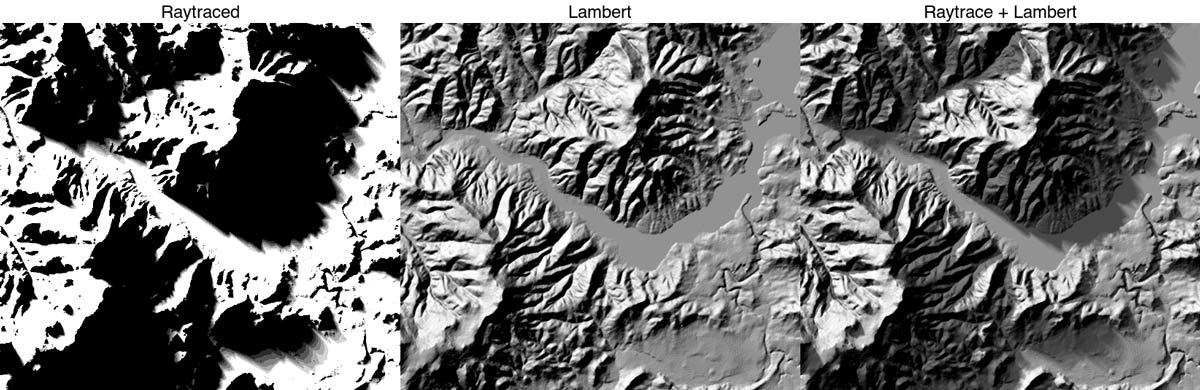
ray_shade), Lambertian reflectance (lamb_shade), and the combined shadow map. The two shadow maps were combined with a new function, add_shadow, that automatically rescales shadow maps so they don’t completely overwhelm the original image.
Implementing Lambertian reflectance involves determining which direction the surface is pointing and taking the dot product between that and the light vector. The intensity is then equivalent to the cosine of the angle difference: zero (the surface directed right at the light) means it has maximum brightness, and 90 degrees or more means the intensity is zero. Looking for an existing function in the R ecosystem that would do this, I found none–but luckily for me, years and years of TA-ing Intro to Physics during my PhD immediately let me see the solution.
Ask the internet how to do something and you’re likely to get a bunch of digital shrugs and maybe—if you’re lucky—a passive aggressive link to a Wikipedia page. Tell the internet you’ve done something—and they’ll tell you exactly what you can do to improve it.
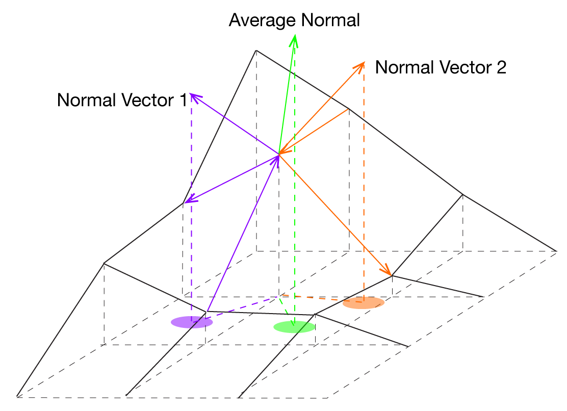
With an elevation matrix on a square grid, we can think of each point having four vectors pointing to it: one from below, one from the left, one from the right, and one from above . The x and y components of each of these vectors are fixed because the grid is fixed–the only component that changes is the z. This component is simply the elevation difference between the two points. By taking the cross product of these vectors, we use the right hand rule to get a vector that points perpendicularly to the surface defined by those vectors. We get two of these surfaces for every point, and we average those vectors to get a single normal vector for that point.
This worked and the effect was cool–but more importantly, it set me up to easily implement everything that came next. When I posted rayshader to Twitter, @ozjimbob quickly combined it with his spherical texture mapping to create a truly gorgeous map. I decided that this would be the niche rayshader would fill–a package to create beautiful topographic maps, with a combination of texture mapping and raytracing.
I couldn’t use his code, as it was too slow on the extremely large elevation matrices I was using. So I had to implement it myself–but luckily, I had already done most of the work. Spherical texture mapping isn’t too hard to explain: imagine you stretched a texture across a sphere surrounding you in the sky. Each point on the surface is facing towards a point on that sphere. All you need to do is figure out which pixel on the sphere your surface is facing, and then color that point appropriately. The color is entirely a function of the normal vector–which we already have a function to calculate! We don’t even need to call any trigonometric functions; once we have the normal vector, the mapping between surface and sphere is just a few multiplications and divisions away.
Here, let’s assume we have a square, (NxN) array representing our texture. The image can either be imported (using an R package like png or jpeg), but more conveniently rayshader now has a create_texture function that programmatically creates texture maps given five colors: a highlight, a shadow, a left fill light, a right fill light, and a center color for flat areas. The user can also optionally specify the colors at the corners, but create_texture will interpolate those if they aren’t given. We need to map the x, y, and z-components of the normal vector to positions on the texture map. We map our z-normal onto the distance from the center R, and the x and y-normals ((n_x) and (n_y)) tell us from what angle around the texture map we sample.
\[ 1 = n_x^2 +n_y^2 +n_z^2\] \[ r = \sqrt{n_x^2 +n_y^2} \] \[ R = (1-n_z) \]
\[ x_{\text{coord}} = R \sin(\theta) = R \frac{-n_x}{r} = R\frac{-n_x}{\sqrt{1-n_z^2}} \]
\[y_{\text{coord}} = R\cos(\theta) = R \frac{n_y}{r} = R\frac{n_y}{\sqrt{1-n_z^2}}\]In order to rotate the direction of the highlight from due north to an angle \(\theta_{\text{light}}\), we apply a rotation transformation to the above coordinates. We also add the coordinates of the center of the texture, and apply the floor function to get the integer coordinates of the color on the texture. \[ X_{\text{image}} = \mathrm{floor}\big( x_{\text{coord}}\cos{\theta_{\text{light}}} - y_{\text{coord}}\sin{\theta_{\text{light}}} + \frac{N}{2}\big)\] \[ Y_{\text{image}} = \mathrm{floor}\big(x_{\text{coord}}\sin{\theta_{\text{light}}} + y_{\text{coord}}\cos{\theta_{\text{light}}} + \frac{N}{2}\big)\]
This is implemented in a function in rayshader called sphere_shade. By inputting the elevation matrix and a texture, you can create beautifully colored maps on which you can layer more shadows from rayshader’s other functions. rayshader also includes 7 built-in palettes: Four inspired by by the palettes of Eduard Imhof c(“imhof1”,“imhof2”,“imhof3”,imhof4”), a desert palette “desert”, a black and white palette “bw”, and one called… 🦄 “unicorn” .
We now have a beautiful textured, rayshaded map (with Lambertian reflectance–thanks, Hacker News commentator!)–but we can improve it even more. The amount of light hitting a surface is not just related to the direct light, but also scattered light from the atmosphere. We can model this with an ambient occlusion model, where the amount of light hitting the surface is also modulated depending on the amount of sky visible from that point. This makes valleys darker than flat areas, due to a much smaller amount of the sky visible, even when you’re in direct sunlight. And we can reuse existing code; we simply use the ray_shade function to raytrace out a short distance in a circle around that point, and check for surface intersections. If no rays intersect the surface, it means the full sky is visible from that point. Otherwise, that point is darkened for each intersecting ray.
There’s still something extremely important missing, however: water. Simply filling in the areas with water with the same color we use for relatively flat surfaces would deprive our map of its most basic job: topographic maps, at their most basic level, should tell us at least two things: where there is land, and where there is water. Bodies of water naturally give maps a sense of scale and breaks up maps into human relatable chunks. Remove the distinction between land and water–well, kid, that’s a nice bump map you have there. So we need some automated way of detecting and adding water to our maps.
Thankfully, we (yet again) have already done most of the work to build a water-detection algorithm when we figured out how to calculate the surface normals. Water is flat, so its surface normal is always pointing straight upwards. If we extract all of the areas that are pointing straight up (with a little wiggle room defined by the user), and then only extract contiguous areas larger than a user-defined minimum area (in order to avoid classifying every small flat area as water), you can easily extract the bodies of water from a map. We can extract this area, and then use the function add_water with a color argument to add a water layer to your map. Matching water colors are provided for each of the built-in palettes included in sphere_shade: just provide the same palette name that you provided when building the original texture map (yes, all palettes have a matching water type… 🦄 ). Otherwise supply your own hexadecimal color. This should be done after calling sphere_shade, but before adding any shadows to your map, otherwise the water will overwrite the shadows you added.
Bodies of water naturally give maps a sense of scale and breaks up maps into human relatable chunks. Remove the distinction between land and water–well, kid, that’s a nice bump map you have there.
Finally, we combine the spherical texturing, raytraced shadows, lambertian reflectivity, ambient occlusion, and water layers all together to create our final image. To do this, we element-wise multiply our R, G, and B channels in the spherical texture map with our shadow matrices. By default, our shadow matrix is scaled from 0 to 1 (0 is complete darkness, 1 is full illumination), but we don’t want to cover up all of the details in the completely shaded areas (0 in all color channels is black). We then rescale the shadow matrices from from 0-1 to a much smaller range (the default in rayshader is 0.7-1.0), so that completely shaded areas won’t be black, just darker. Rayshader has an add_shadow function that does just that: input a shadow map and the map to be shaded, and it rescales and multiplies them correctly. This works at any stage of the process: you can use add_shadow to combine shadow matrices as well as texture maps, in any order.
elmat %>%
  sphere_shade() %>%
  add_water(detect_water(elmat)) %>%
  add_shadow(ray_shade(elmat,lambert=FALSE)) %>%
  add_shadow(lamb_shade(elmat)) %>%
  add_shadow(ambient_shade(elmat)) %>%
  plot_map()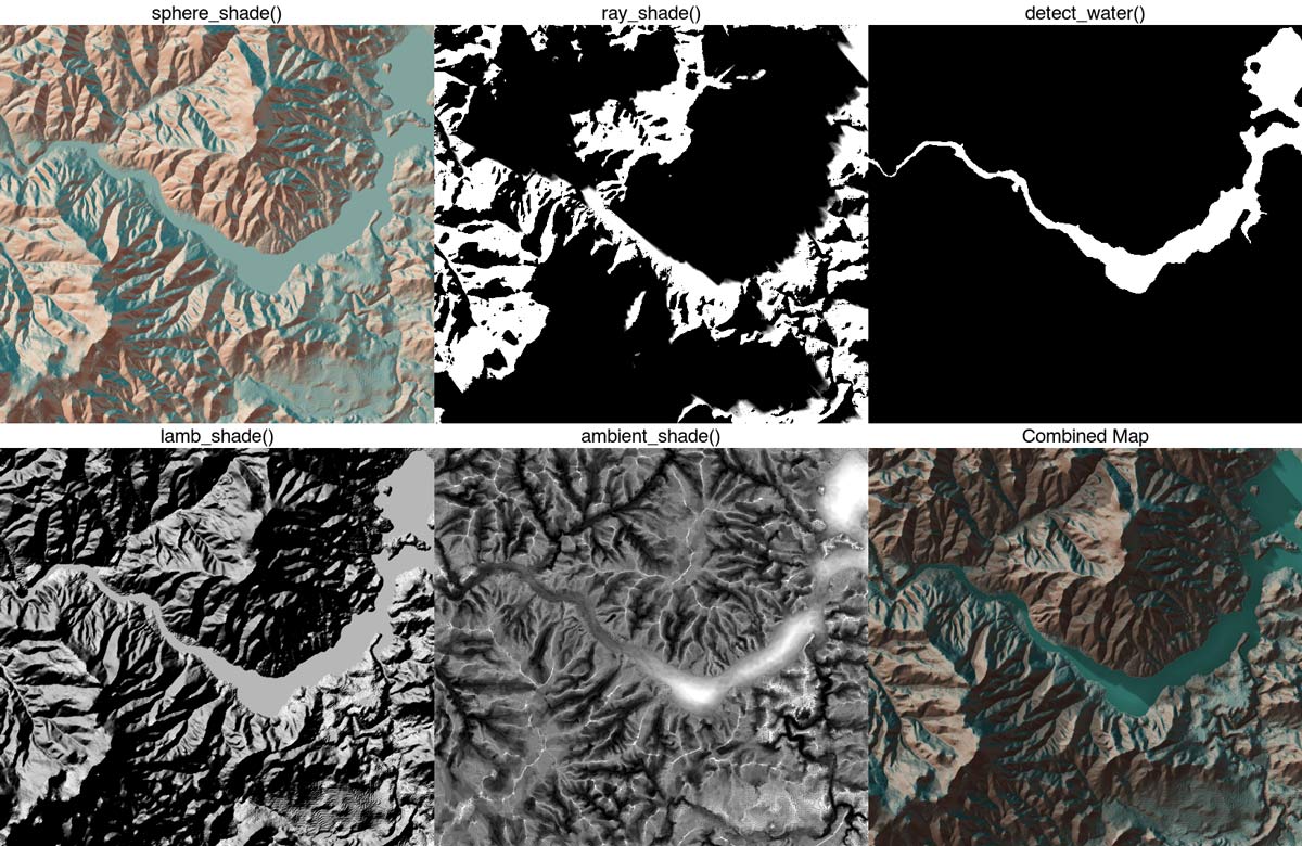
rayshader. With the add_shadow and add_water functions, we can easily add more layers to our hillshade.
One of the lessons I’ve learned during all of this is the importance of releasing as soon as you have a “minimally viable product.” I had a few ideas of where next to take the project, but seeing other people use it immediately drove the development to a place I never even considered (although I’m still going to develop those ideas I originally had in mind). If you want to try it yourself but don’t have any topographic data on hand (and let’s face it–the volcano data set is pretty boring), here’s the test data set I’ve been playing with–it includes water (zip file, 620Kb). Or you could try the elevatr package by Jeff Hollister. It can easily load topographic data from Amazon’s tile service, and you can get rolling as easy as this:
library(rayshader)
library(elevatr)
library(magrittr)

#from the .tif file
eltif = raster_to_matrix("~/path/to/file/dem_01.tif")

#or from the elevatr package
elevation <- get_elev_raster(lake, z = 11, src = "aws")

elmat2 = matrix(raster::extract(elevation,raster::extent(elevation)),
                nrow=ncol(elevation),ncol=nrow(elevation))

elmat2 %>%
  sphere_shade() %>%
  add_water(detect_water(elmat2)) %>%
  plot_map()
As for the latest version of rayshader, see the link below–I look forward to seeing what cool maps you can make with it!
And if you want to see more cool stuff, follow me on Twitter and sign up for my newsletter for the latest updates on rayshader!
Follow @tylermorganwall
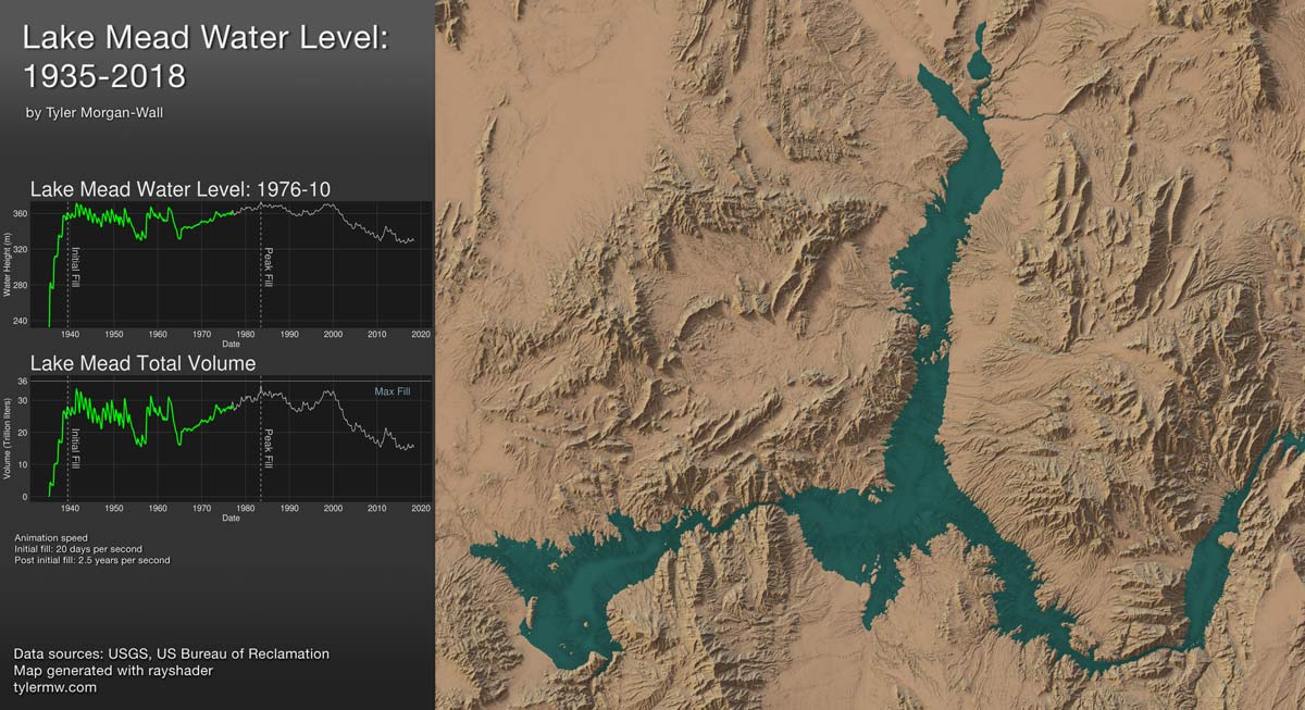
Creation of the featured Lake Mead figure:
The creation of this figure started by going to the USGS map viewer website and downloading topographic data for the area. This gave me the size of the lake at full capacity, which I was then able to extract the lake surface with the detect_water function in rayshader. I then found bathymetric (undersea elevation) data of Lake Mead collected from sonar data gathered in 2001 by the USGS (thanks again!). This gave me the topographic information of the area sans water, although of much lower resolution than the actual topographic map. You might notice jumps in the animation: those occur every 30 feet, which was the sampling resolution of the sonar.
I then aligned the bathymetric map with the lake surface extracted from the other dataset. To raise the water level, I replaced everything under the lake surface and under a set height with that height. This just involved subsetting the elevation matrix for those heights under the set limit, and replacing them if they also were in the lake area (defined by the mask) elmat[mask == 1 & elmat . I did this in half-meter increments from no water (232m above sea level) to full depth (374m above sea level), and output an image for each height.
I then scraped the historical monthly lake levels from this US Bureau of Reclamation website to determine the water level since the Hoover Dam was built. I then wrote a script to create images in order of the the correct height for each date. The first few years when the lake was filling was much more interesting than the following 80 years, so I interpolated between those data points to slow down the animation and emphasize that portion.
I extracted the volume of the lake by taking the sum of the total difference between the new adjusted lake height map and the original map (which gives the elevation difference in meters), and multiplying it by 100 m^2 (10mx10m area per data point).
For the aesthetic portion, I used the “desert” built-in palette in sphere_shade. I used the detect_water function to determine where the waterline was, and replaced the color on that area with the “imhof2” palette (there’s a matching lighter palette for “desert”, but it didn’t look as nice with the ambient occlusion layer added under the water). I added a raytraced layer with add_shadow, ray_shade, and ambient_shade. This would take a long time to do for every single frame, so I also used the lake surface to tell ray_shade to only update the raytraced shadows under the lake surface. The ambient_shade layer I only calculated once and added on top of the water layer, to show the topographic features below the surface. Finally, I combined the map with plots using ImageMagick showing the water level as a function of date, and total water volume (computed by taking the volume of water under the water level). I then used ffmpeg to create a video out of all 1759 images.