The Virtual Tilt Card: Raytracing Lenticular Prints with rayrender
Note: This post is also marks the release of rayrender 0.3.0: to see what new features are included (and there are many), head to the bottom of the post.
When I was a kid back in the 1990s, cereal companies used a clever little marketing trick to get their wares in our parents carts: literally just bribing children. With “prizes.” Little plastic submarines, spoons that morphed from Ectocooler green to Wild and Crazy Kids purple when dipped in milk, and most often of all: collectable trading cards. Although these cards were neither collectable nor traded by any child not holding a SAG card, they became a mainstay of the cereal prize economy . And because these corporations knew no kid who had access to 50 whole channels of cable television would ever care about a stupid little card with a picture of Simba on it, they added one critical feature: They made the characters move when you wiggled them back and forth.
The tilt card. Kid crack.
And truthfully, the 90s were the last time I had put any thought into those real-world animated GIFs. That is, until this past January, when a mashup visualization I made using #plottertwitter and rayshader got this response from Hadley Wickham:
Random thought: could you model lenticular printing in rayshader? ie. make a virtual version of https://t.co/jGZvmfAZIr
— Hadley Wickham (@hadleywickham) February 13, 2019
My first thought: “What the heck is lenticular printing?” One wikipedia page later I had my answer: it’s the technology that powered all of the cereal tilt cards of my youth. How they work: you pack a grid of tiny cylindrical lenses on top of interleaved strips of multiple images. The lenses focus the light at certain angles onto a one of those strips, magnifying it to the size of the lens. As you change the angle, the strip at the focal point changes and the image shifts, giving you a little animation.
This effect wasn’t possible with rayshader, since it cannot model refractive materials… but a month later, I started work on rayrender, a fully-featured pathtracer in R. And that package WAS capable, in theory, of modelling this effect. Which Hadley (a month later) was quick to pick up on:
Am I going to get the rayshaded animated lenticular gifs that I have always dreamed of?????
— Hadley Wickham (@hadleywickham) February 28, 2019
Of course, I had to add a couple of features: cylinders, the ability to render only certain subtended arc of those cylinders, and support for textures. And with the latest version (v0.3.0) of rayrender, all those features are now included! So how do you turn a GIF into a virtual lenticular print? Let’s first build a toy example to show how lenticular lenses work.
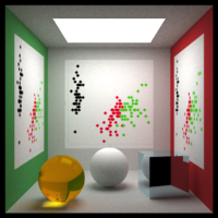
(For a more basic introduction to rayrender, see this previous blog post.)
First, we’ll interleave strips of three colors: red, green, and blue. We do this by using the xy_rect object, which creates a rectangle in the xy-plane. We’ll use the add_object function to build the scene, and place three groups of them in the middle of the box.
library(rayshader)
library(rayrender)

strip_width = 50/3
interlaced_rects = list()
offsets = c(-50,0,50)

for(i in 1:3) {
  xy_rect(x = 555/2 + strip_width + offsets[i], y = 200, z = 555/2,
          ywidth = 400, xwidth = strip_width,
          material = diffuse(color="red")) %>%
    add_object(xy_rect(x = 555/2 + offsets[i], y = 200, z = 555/2,
                       ywidth = 400, xwidth = strip_width,
                       material = diffuse(color="green"))) %>%
    add_object(xy_rect(x = 555/2 - strip_width + offsets[i], y = 200, z = 555/2,
                       ywidth = 400, xwidth = strip_width,
                       material = diffuse(color="blue"))) ->
  interlaced_rects[[i]]
}
#the do.call(rbind, ...) function just turns our list into a data frame.
interlaced_rect_scene = do.call(rbind,interlaced_rects)

initial_scene = generate_cornell(lightintensity = 20) %>%
  add_object(interlaced_rect_scene)

render_scene(initial_scene, parallel=TRUE, width = 800, height = 800, samples = 40,
               ambient_light = FALSE, tonemap = "reinhold", aperture = 0)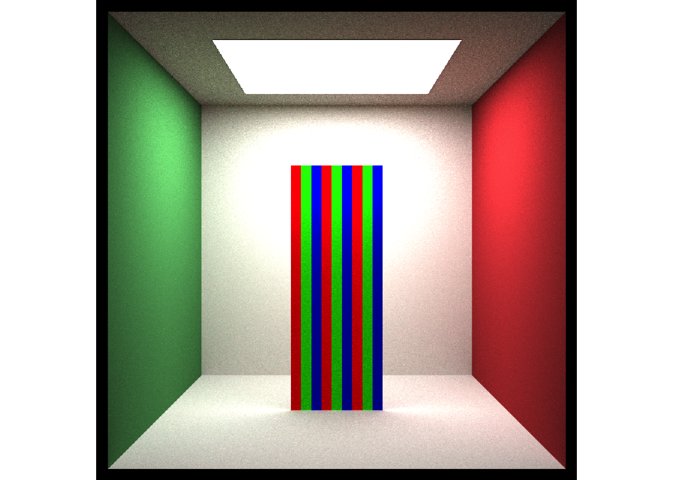
Now, we stick a lenticular lens in front of them. This lens will be a quarter of a cylinder, which we will specify with the min_phi and max_phi arguments. The radius will be the width of the three interleaved columns, and the center of the cylinder will be centered one radial unit away from the surface. We will also rotate the lens to face outwards.
radius = 3*strip_width/sqrt(2)
lenticular_sheet = cylinder(x=555/2+offsets[1], y = 200, z = 555/2-radius,
                      length = 400, phi_min = 225, phi_max = 315, radius = radius,
                      material = dielectric(color="white")) %>%
  add_object(cylinder(x=555/2+offsets[2], y = 200, z = 555/2-radius,
                      length = 400, phi_min = 225, phi_max = 315, radius = radius,
                      material = dielectric(color="white")))  %>%
  add_object(cylinder(x=555/2+offsets[3], y = 200, z = 555/2-radius,
                      length = 400, phi_min = 225, phi_max = 315, radius = radius,
                      material = dielectric(color="white")))

scene_with_lens = initial_scene %>%
  add_object(lenticular_sheet)

#Create the animation flying around the scene to demonstrate the geometry.
t = 1:360*pi/180
xval = 555/2 + 100 * sin(t)
zval = -300 + 500 * cos(t)
lookaty = 239 - 39 * cos(t)
lookfromy = 278 + 100 + 100 * cos(t)
fovvec = 62.5 + 22.5 * cos(t)

for(i in 1:360) {
   render_scene(scene_with_lens, parallel=TRUE, width = 600, height = 600,
                samples = 400, ambient_light = FALSE, tonemap = "reinhold",
                aperture = 0, fov=fovvec[i],
                filename = glue::glue("toyexample{i}"),
                lookfrom = c(xval[i],lookfromy[i],zval[i]),
                lookat = c(555/2,lookaty[i],555/2-radius/2))
}

system("ffmpeg -framerate 30 -pix_fmt yuv420p -i toyexample%d.png toyexample.mp4")In raytracing, we generate our image of the scene by shooting rays out of the camera. Imagine shooting rays out of our eyes to sample the colors and lighting of the scene. At certain angles, all of those rays are refracted by the dielectric cylinder onto a single strip, which makes the lens appear that color (ignoring the reflection term). When we are at an angle where some of the rays hit one strip and some hit an adjacent strip, we can see both colors in a cylinder. This is what gives lenticular prints their characteristic gradual transition between frames.
Taking that into consideration, if we tilt the object back and forth, we can selectively focus on just one of the color strips. In Figure 5 below, I rock the toy example back and forth 25 degrees. To do this, we use the group_objects() function to group all of the elements of the tilt card together, and the group_angle argument to rotate them all together (around the group pivot point). Note how the lenses only focus on one of the strips at certain angles.
tilt_angle = 25 * sin(t)
for(i in 1:360) {
   angled_scene_with_lens = generate_cornell(lightintensity = 20) %>%
     add_object(
       group_objects(interlaced_rect_scene %>%
           add_object(lenticular_sheet),
           pivot_point = c(555/2,555/2,555/2-radius/2),
           group_angle = c(0,tilt_angle[i],0)
         )
       )

     render_scene(angled_scene_with_lens, parallel=TRUE,
                  width = 600, height = 600, samples = 400,
                  ambient_light = FALSE, tonemap = "reinhold",
                  aperture = 0, fov=40,
                  filename = glue::glue("toyexampletilt{i}"))
}

for(i in 1:360) {
   angled_scene_with_lens = generate_cornell(lightintensity = 20) %>%
     add_object(
       group_objects(interlaced_rect_scene %>%
           add_object(lenticular_sheet),
           pivot_point = c(555/2,555/2,555/2-radius/2),
           group_angle = c(0,tilt_angle[i],0)
         )
       )

     render_scene(angled_scene_with_lens, parallel=TRUE,
                  width = 150, height = 150,
                  samples = 400, ambient_light = FALSE,
                  tonemap = "reinhold",
                  aperture = 0, fov=fovvec[1], clamp_value = 10,
                  lookfrom = c(xval[1],lookfromy[1],zval[1]),
                  lookat = c(555/2,lookaty[1],555/2-radius/2),
                  filename = glue::glue("toyexampletiltabove{i}"))
}

#Create the animation with the overhead inset, using ImageMagick on the command line.
system("for i in {1..360}; do convert toyexampletilt$i.png '(' toyexampletiltabove$i.png -bordercolor '#000000' -border 5 ')' -geometry +400+50 -composite combinedtoy$i.png; done;")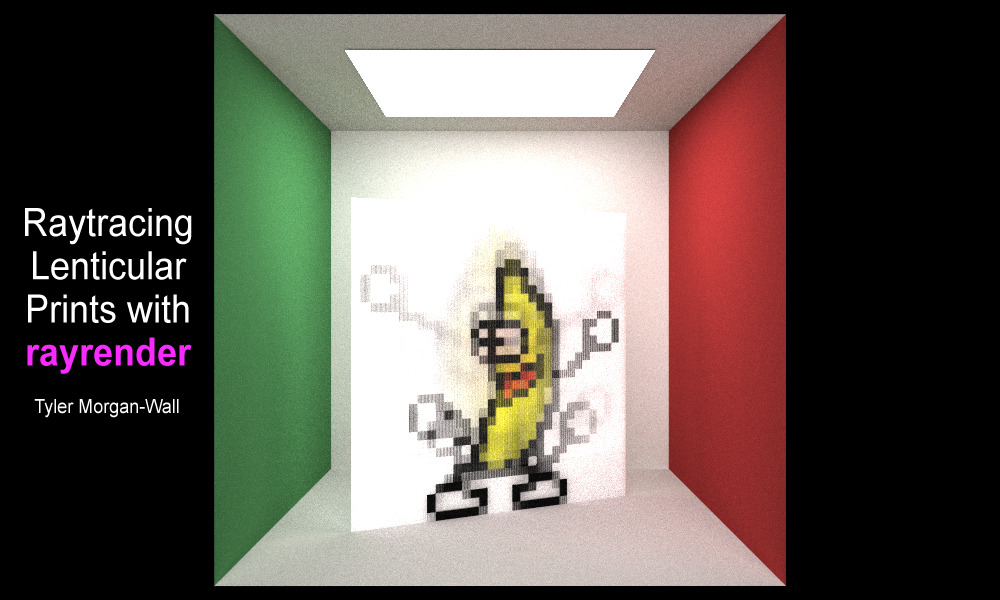
system("ffmpeg -framerate 30 -pix_fmt yuv420p -i combinedtoy%d.png combinedtoy.mp4")Now, let’s demonstrate this on a much larger scale: instead of interleaving three colors, we are going to interleave frames of a GIF. The GIF of honor: this dancing banana (which will be familiar to millennials, and probably only known by Gen Z as a Fortnite dance or something):
Figure 6: In 2019, it’s organic single-origin almond spread and raspberry compote time. With a baseball bat.
This involves taking each column of pixels from the full animation and stacking them side-by-side with each subsequent frame. If our GIF has N frames, this means our final image will be N times wider than the original, since all frames are now present in the single (non-moving) output image. Here, I hack together a for loop to do this quickly–there are definitely more elegant ways to interleave matrices and arrays, but this one required zero thought and worked on the first try :)
bananas = list()
for(i in 1:8) {
  bananas[[i]] = aperm(png::readPNG(glue::glue("~/Desktop/bananatest/banana{i}.png")), c(2, 1, 3))
}
#Dimensions of banana gif is 378x401--create a 4 layer array with space for all 8 frames.
tempbananas = array(0, dim = c(378*8, 401, 4))

#Interleave the frames:
counter = 1
counter2 = 1
for(i in 1:(378*8)) {
  if(counter2 > 8) {
    counter2 = 1
  }
  if(counter2 == 1) {
    tempbananas[i,,] = bananas[[1]][counter,,]
  } else if(counter2 == 2) {
    tempbananas[i,,] = bananas[[2]][counter,,]
  } else if(counter2 == 3) {
    tempbananas[i,,] = bananas[[3]][counter,,]
  } else if(counter2 == 4) {
    tempbananas[i,,] = bananas[[4]][counter,,]
  } else if(counter2 == 5) {
    tempbananas[i,,] = bananas[[5]][counter,,]
  } else if(counter2 == 6) {
    tempbananas[i,,] = bananas[[6]][counter,,]
  } else if(counter2 == 7) {
    tempbananas[i,,] = bananas[[7]][counter,,]
  } else {
    tempbananas[i,,] = bananas[[8]][counter,,]
    counter = counter + 1
  }
  counter2 = counter2 + 1
}
rayshader::plot_map(tempbananas, rotate = 90)Now, we load this image as a texture onto a square in a rayrender scene. I’ll put it inside a Cornell box, because that’s just what you do (when you’re raytracing).
initial_scene = generate_cornell(lightintensity = 20) %>%
  add_object(yz_rect(x = 555/2, y = 200, z = 555/2, ywidth = 400, zwidth = 400,
                     material = diffuse(image_texture = tempbananas), angle = c(90, 90, 0)))

render_scene(initial_scene, parallel=TRUE, width = 800, height = 800, samples = 400,
               ambient_light = FALSE, tonemap = "reinhold", aperture = 0)
## Setting default values for Cornell box: lookfrom `c(278,278,-800)` lookat `c(278,278,0)` fov `40` .
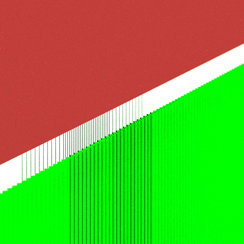
Right now there’s nothing special about the above–it’s simply a texture on an square. The magic comes when we slide our array of cylindrical lenses in front of this interlaced image. We’ll use the same spacing as above–one cylindrical lens will be in front of 8 strips, as there are 8 frames in our gif. Since the width of our rectangle is 400 units wide and the original image is 378 pixels across, our pixel width will be () units wide. The radius of the cylinder will be (r = ), and we will subtend a 90 degree arc in front of the image. Here’s an image looking down the side, showing off the geometry (the lenses are tinted green in order to highlight their geometry):
pix_width = (1/378) * 400
radius = pix_width/sqrt(2)

cyllist = list()
for(i in 1:378) {
  cyllist[[i]] = cylinder(x=200-i*radius*sqrt(2),z = -radius , y=0,
                          length = 400, phi_min = 225, phi_max=315,
                          radius=radius,angle=c(0,0,0),
                          material = dielectric(color="green"))
}

do.call(rbind,cyllist) -> cyldf

look_from_above = generate_cornell(lightintensity = 10) %>%
    add_object(
      group_objects(
        yz_rect(ywidth=400,zwidth=400,
                material= diffuse(image_texture = tempbananas),
                angle = c(90,90,0)) %>%
               add_object(cyldf),
        pivot_point = c(0, 0, 0),
        group_translate = c(555/2,200,555/2), group_angle = c(0,0,0)
        )
      ) %>%
    add_object(xy_rect(x=555/2,y=555/2,z=-1000,
                       xwidth=1000, ywidth=1000,
                       material = diffuse(lightintensity = 10, implicit_sample = TRUE),
                       flipped = FALSE))

render_scene(look_from_above, parallel=TRUE, width=800, height=800,
             samples = 100, fov = 1,
             lookat = c(555/2,400,555/2-1), tonemap = "reinhold",
             lookfrom = c(555/2+200,410,555/2-20), clamp_value = 10,
             ambient_light = FALSE, aperture = 0.5)
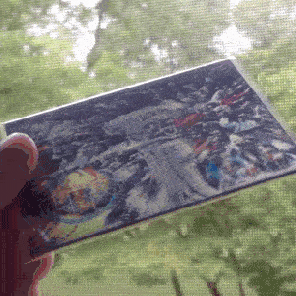
Finally, to generate the virtual lenticular print, we simply tilt the card back and forth. This shifts the focal point of each lens onto a single strip (representing a single frame of the gif) and makes the banana dance. You can see the characteristic “blending” of one frame to another inherent to lenticular printing.
Dance, banana, dance!
t = 1:360
angle = -45 * cos(t*pi/180)
x = 10 * sin(angle*pi/180)
z = 10 * cos(angle*pi/180)
for(i in seq(1, 360,1)) {
  banana_scene = generate_cornell(lightintensity = 10) %>%
    add_object(
      group_objects(
          yz_rect(ywidth=400,zwidth=400,
                  material= diffuse(image_texture = tempbananas),
                  angle = c(90,90,0)) %>%
          add_object(cyldf),
        pivot_point = c(0, 0, 0),
        group_translate = c(555/2,200,555/2),
        group_angle = c(0,angle[i],0)
        )
      ) %>%
    add_object(xy_rect(x=555/2,y=555/2,z=-1000, xwidth=1000, ywidth=1000,
                       material = light(intensity = 10),
                       flipped = FALSE))

    render_scene(banana_scene, parallel=TRUE, width=600,height=600,
                 samples=100, clamp_value = 15,
                 lookat = c(555/2,555/2,555/2),
                 filename = glue::glue("bananadance{i}"),
                 ambient_light = FALSE, tonemap = "reinhold",aperture = 0

system("ffmpeg -framerate 30 -pix_fmt yuv420p -i bananadance%d.png bananadance.mp4")
}So the next time someone spouts some nonsense about R just being for statisticians and academics, you can correct them: R isn’t just a language for statistical computing, it’s also a language to make bananas dance in the most roundabout way possible. I expect they might not have a response.
Like what you read? Sign up for my listserve to get piping-hot fresh content into your inbox!
Package update: rayrender 0.3.0!
This post also marks the 0.3.0 release of rayrender! This is a fairly substantial release, and includes the following:
-
Added .obj file support (with diffuse textures). Also included is a 3D model of the letter “R”, which can be loaded by calling the function
r_obj()intoobj_model(). - Added multicore progress bars using RcppThread.
- Added triangle primitive. Supports per-vertex color and normals.
- Added disk primitive. Supports an inner radius term.
- Added cylinder primitive. Supports rendering only a subtended arc of the cylinder.
- Added segment primitive (cylinder defined by a start and end point).
- Added ellipsoid primitive.
- Added pig() function, which returns a model built out of primitives. Oink.
- Added spherical background images.
- Added bounding box intersection algorithm from “A Ray-Box Intersection Algorithm and Efficient Dynamic Voxel Rendering” for more consistent BVH intersections.
- Added transformation to scale primitives (or grouped primitives) in any (or multiple) axes.
-
Added HDR tonemapping options in
render_scene() - Added option to set Cornell box colors.
- Bug fixes (of course)
For more information, usage examples, and documentation, check out the package website: rayrender.net.
r check out the Github page directly: