Getting Started with Rayrender: Forging the R Sword
In mid-February, I found myself staring at the computer screen with a weekend free and a choice to make. After three months working on rayshader to put together and practice a presentation for RStudio::conf(2019), build the package a website, and bring life to an interactive rayshading Twitterbot–I found myself feeling the smallest tinge of “burn out”. Not enough to say ik ben op, as the Dutch so poetically put it–but I had been working on the same project for a while and needed something new and exciting in my life . I wanted to take a little break and tackle a new problem–one that might not provide me with any immediate benefit, but might help rayshader in the long run.
So I decided to build a raytracer.
Although “rayshader” has “ray” in the name, it only uses “ray tracing” in the most basic sense: it traces rays from points on an elevation matrix to bake a shadow map onto the surface of an object. The simplicity of the method means implementing techniques like ambient occlusion is trivial, and baking the shadow map into the texture is great for fast, interactive plotting–but you would never confuse the output of rayshader for a pathtracer . So I had been meaning to dive deeper into real raytracing in order to one day bring a higher quality renderer to rayshader.
render_depth() function certainly helps narrow that divideAnd luckily for me, there’s never been a better time to learn about raytracing!
Last year, two resources were released free-of-charge that made learning about raytracing immensely easier: Matt Pharr’s Physically Based Rendering: From Theory To Implementation textbook, and Peter Shirley’s Ray Tracing in One Weekend three book series. The former was great as a reference, but a bit unwieldy as a way to introduce yourself to the subject. Peter Shirley’s books, however, hit the pedagogical sweet spot (in my opinion): easily understandable and concise code, plain English explanations of what the code is doing, and a built-in system of student feedback by immediately diving into producing cool output. But more importantly, I could see right away how I could use what he taught to build a raytracer in R.
And luckily for me, there’s never been a better time to learn about raytracing!
Enter: rayrender.
Rayrender is an R package that uses raytracing to render scenes consisting of spheres, cubes, and 2D planes. The “scene” is just a tibble where each row contains all the information required to draw on object, and the collection of such objects is passed to the render_scene() function to draw an image (or save an image to file). Similarly to how you build a map in rayshader, you build the scene in layers and compose them all together with the add_object() function. Here, we generate a large sphere as the “ground” and then place a grey sphere on top of it.
#Install the package if you haven't already
#remotes::install_github("tylermorganwall/rayrender")
library(rayrender)

scene = sphere(y=-1001,radius=1000,material = lambertian(color = "#ccff00")) %>%
  add_object(sphere(material=lambertian(color="grey50")))
render_scene(scene)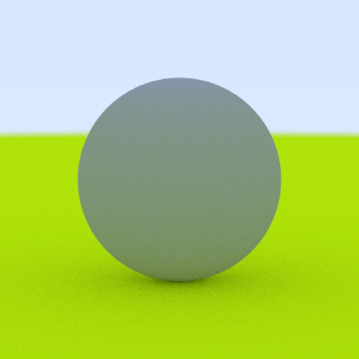
Not very exciting? Okay, let’s replace the ground with something a little more interesting. How about a checker pattern? And let’s make the ball a light reddish color. The API is designed so that each object accepts a material argument, to which you pass the output of one of the material functions: lambertian, metal, or dielectric.
scene = sphere(y=-1001,radius=1000,
               material = lambertian(color = "#ccff00",checkercolor="grey50")) %>%
  add_object(sphere(material=lambertian(color="#dd4444")))
render_scene(scene, width=500, height=500, samples=500)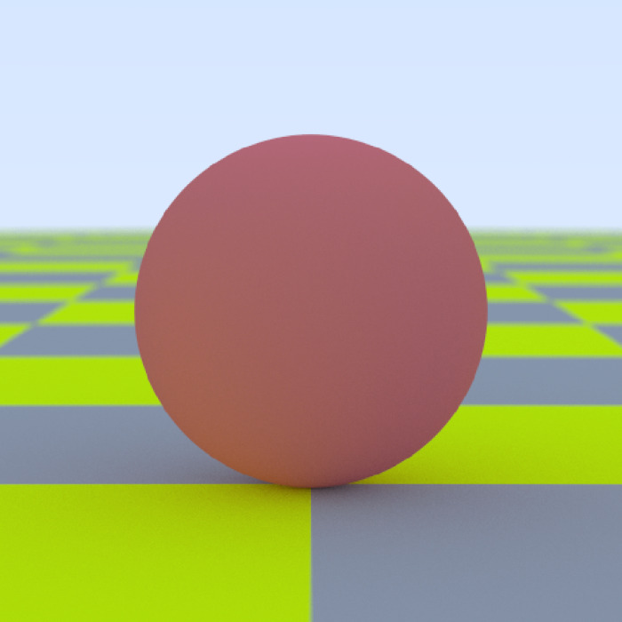
You might be thinking: “Wait. This scene doesn’t look like anything special. 🤔Aren’t raytracers supposed to have floating metallic spheres and glass balls everywhere?”
scene = sphere(y=-1001,radius=1000,
               material = lambertian(color = "#ccff00",
                                     checkercolor="grey50")) %>%
  add_object(sphere(material=lambertian(color="#dd4444"))) %>%
  add_object(sphere(z=-2,material=metal())) %>%
  add_object(sphere(z=2,material=dielectric()))
render_scene(scene,width=500, height=500, samples=500,
             fov=40,lookfrom=c(12,4,0))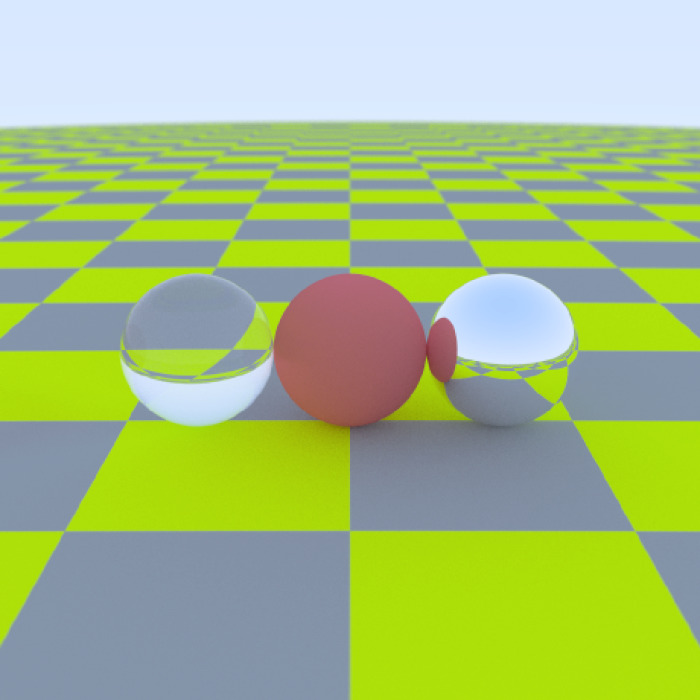
You need not worry. Glass to the left, and metal to the right. Here, I changed the sphere from the default diffuse material to glass and metal by specifying a different material argument in the object function.
🤔 “Aren’t raytracers supposed to have floating metallic spheres and glass balls everywhere?”
Now, one of the coolest thing about raytracers is how easy it is to add realistic lighting to the scene–and we can do that simply by setting the lightintensity argument in a lambertian material to a positive number. The greater the intensity, the brighter the light. Adding an emissive object turns off the ambient lighting, although the user can override this by setting ambient_light = TRUE in render_scene(). Here, the scene is plotted twice: once far away to show the overhead position of the light, and once up close to show its effect on the spheres.
scene = sphere(y=-1001,radius=1000,
               material = lambertian(color = "#ccff00",
                                     checkercolor="grey50")) %>%
  add_object(sphere(material=lambertian(color="#dd4444"))) %>%
  add_object(sphere(z=-2,material=metal())) %>%
  add_object(sphere(z=2,material=dielectric())) %>%
  add_object(sphere(x=-20,y=30,radius=20,material=lambertian(lightintensity = 3)))

par(mfrow=c(1,2))

render_scene(scene,fov=40, width=500, height=500, samples=500,
             lookfrom=c(50,10,0),parallel=TRUE)
render_scene(scene,fov=30, width=500, height=500, samples=500,
             lookfrom=c(12,4,0),parallel=TRUE)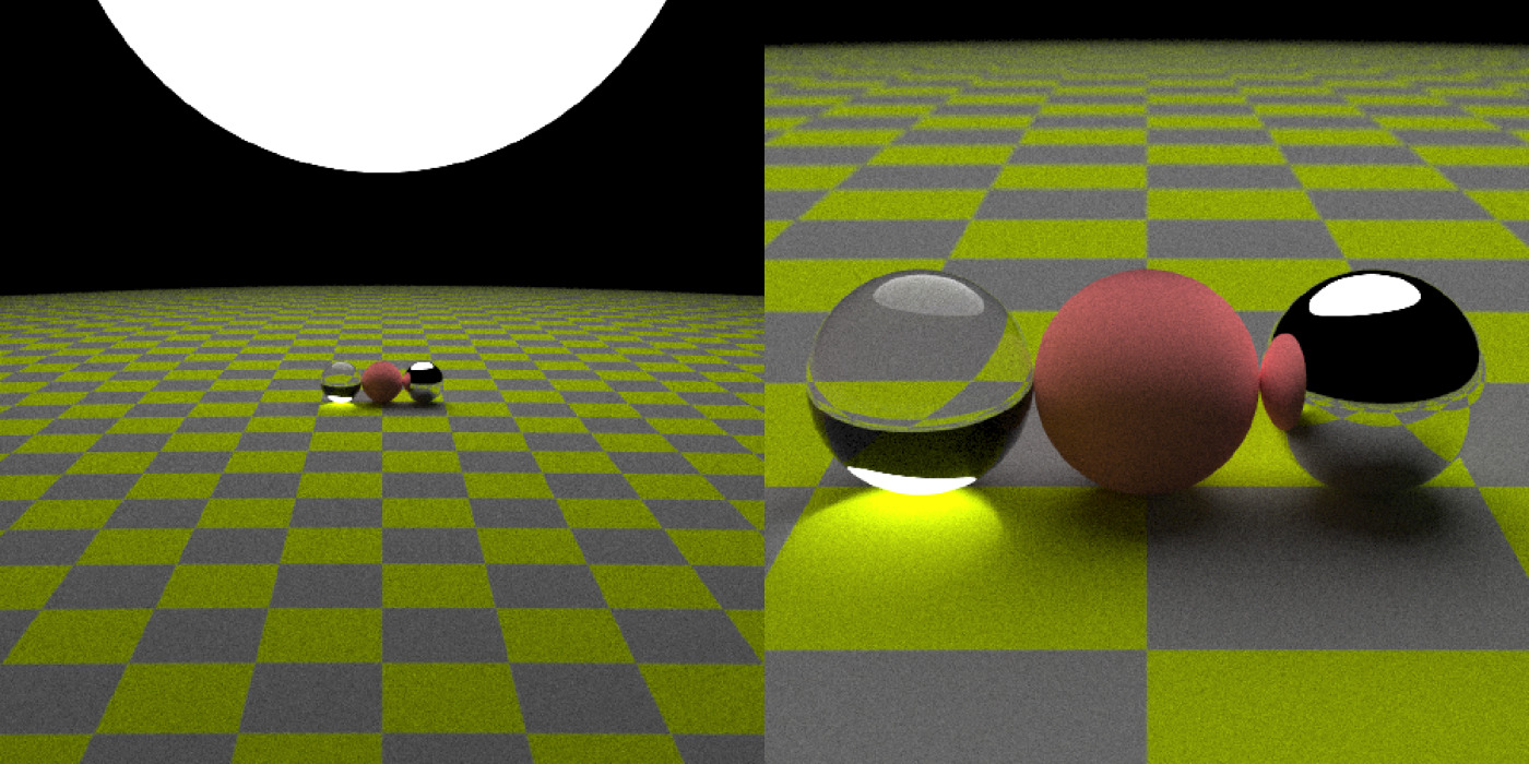
rayrender also supports motion blur for spheres. Let’s give each sphere a velocity (each sphere here is traveling in a different direction):
scene = sphere(y=-1001,radius=1000,
               material = lambertian(color = "#ccff00",
                                     checkercolor="grey50")) %>%
  add_object(sphere(material=lambertian(color="#dd4444"),
                    velocity=c(-2,0,0))) %>%
  add_object(sphere(z=-2,material=metal(),
                    velocity=c(0,1,0))) %>%
  add_object(sphere(z=2,material=dielectric(),
                    velocity=c(0,0,0.5))) %>%
  add_object(sphere(x=-20,y=30,radius=20,
                    material=lambertian(lightintensity = 3)))

par(mfrow=c(1,1))

render_scene(scene,fov=40, width=500, height=500, samples=500,
             lookfrom=c(12,4,0),parallel=TRUE)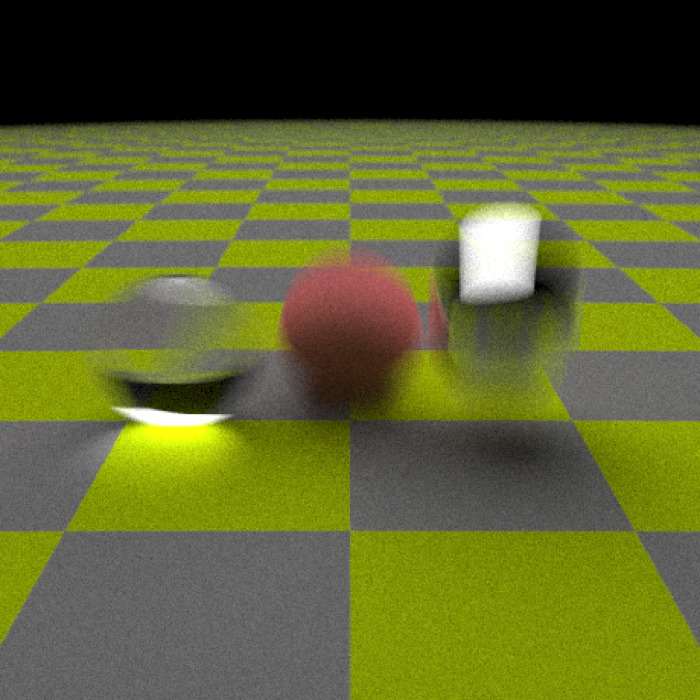
Okay, spheres are nice–how about cubes? Let’s turn the glass object green and lift all the objects off the ground to highlight the light transmission.
scene = sphere(y=-1001,radius=1000,
               material = lambertian(color = "#ccff00",
                                     checkercolor="grey50")) %>%
  add_object(cube(width=2,y=0.1,
                  material=lambertian(color="#dd4444"))) %>%
  add_object(cube(z=-2.2,y=0.1,width=2,
                  material=metal())) %>%
  add_object(cube(z=2.2,y=0.1,width=2,
                  material=dielectric(color="green"))) %>%
  add_object(sphere(x=-20,y=30,radius=20,
                  material=lambertian(lightintensity = 5)))

render_scene(scene,fov=40, width=500, height=500, samples=500,
             parallel=TRUE,lookfrom=c(12,4,0))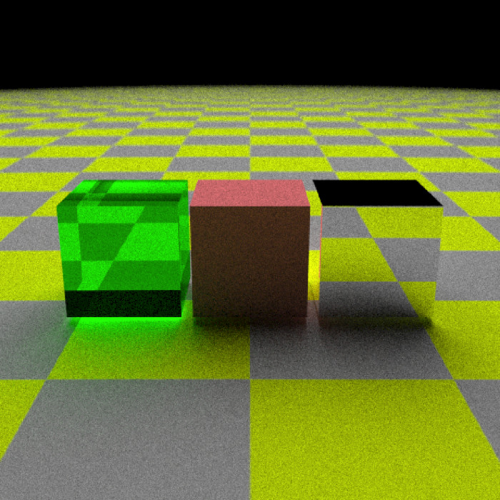
Now let’s build something more substantial: how about a pyramid, with a golden block on top? We’ll also change the ground to be a procedurally generated dirt pattern, using the generate_ground() function (which just wraps the sphere function in a nice interface). We’ll view the pyramid from all four cardinal angles and create a grid of images.
scene = generate_ground(depth=-0.5,spheresize=1000,
                        material=lambertian(color="#000000",noise=1/10,
                                            noisecolor = "#654321")) %>%
  add_object(sphere(x=-20,y=30,radius=20,
                    material=lambertian(lightintensity = 3)))
firstlayer = c(-1.5,-0.5,0.5,1.5)
secondlayer = c(-1,0,1)
thirdlayer = c(-0.5,0.5)

firstlayerdf = expand.grid(x=firstlayer,z=firstlayer,y=0)
secondlayerdf = expand.grid(x=secondlayer,z=secondlayer,y=1)
thirdlayerdf = expand.grid(x=thirdlayer,z=thirdlayer,y=2)

pyramid_positions = rbind(firstlayerdf,secondlayerdf,thirdlayerdf)

for(i in 1:nrow(pyramid_positions)) {
  scene = add_object(scene,cube(x=pyramid_positions$x[i],
                                y=pyramid_positions$y[i],
                                z=pyramid_positions$z[i],
                                material = lambertian(color="tan")))
}

scene = scene %>% add_object(cube(y=3,material = metal(color="gold",fuzz=0.2)))

par(mfrow=c(2,2))
render_scene(scene,fov=40, width=500, height=500, samples=500,
             parallel=TRUE, lookfrom=c(-12,6,0),lookat = c(0,1,0))
render_scene(scene,fov=40, width=500, height=500, samples=500,
             parallel=TRUE, lookfrom=c(0,6,12),lookat = c(0,1,0))
render_scene(scene,fov=40, width=500, height=500, samples=500,
             parallel=TRUE, lookfrom=c(12,6,0),lookat = c(0,1,0))
render_scene(scene,fov=40, width=500, height=500, samples=500,
             parallel=TRUE, lookfrom=c(0,6,-12),lookat = c(0,1,0))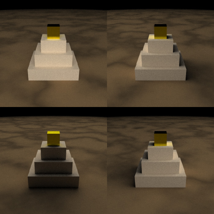
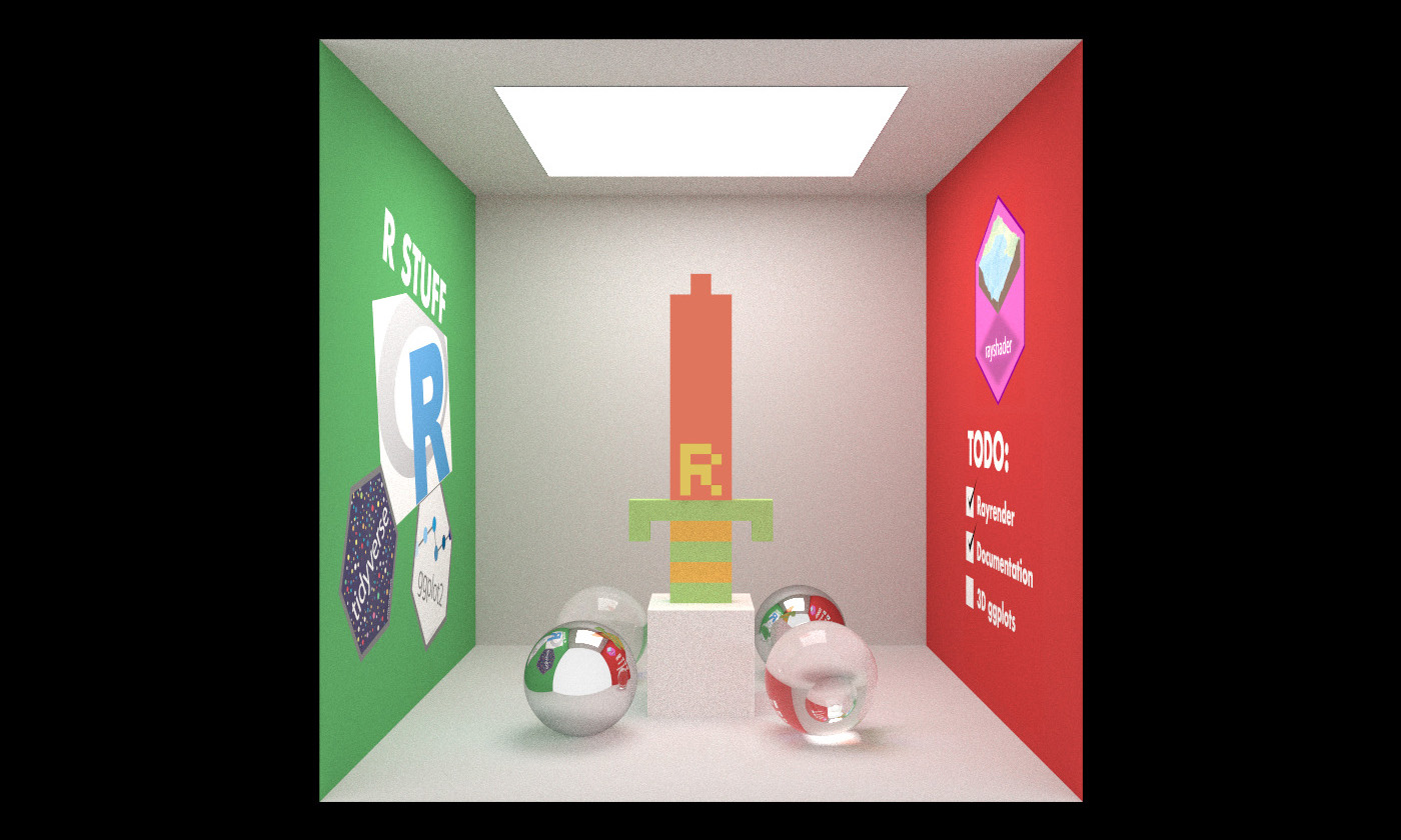
Finally, now that we know how to compose a scene: Let’s forge the R sword, modeled after Link’s wooden sword in the original NES Zelda. We’ll start by creating a matrix that uses a number to represent each separate material/color on the sword. There will be three different materials: a bronze metal for the blade, a green lambertian material for the guard and hilt, and a yellow lambertian for the stripes on the hilt. We will then loop through the matrix and add the appropriate material to the scene when there is a non-zero entry in the matrix.
scene = generate_ground(depth=0,spheresize=1000,
                        material=lambertian(color="#000000",
                                            noise=1/10,
                                            noisecolor = "#654321")) %>%
  add_object(sphere(x=-60,y=55,radius=40,
                    material=lambertian(lightintensity = 8)))

sword = matrix(
c(0,0,0,1,0,0,0,
  0,0,1,1,1,0,0,
  0,0,1,1,1,0,0,
  0,0,1,1,1,0,0,
  0,0,1,1,1,0,0,
  0,0,1,1,1,0,0,
  0,0,1,1,1,0,0,
  0,0,1,1,1,0,0,
  0,0,1,1,1,0,0,
  0,0,1,1,1,0,0,
  0,0,1,1,1,0,0,
  2,2,2,2,2,2,2,
  2,0,3,3,3,0,2,
  0,0,2,2,2,0,0,
  0,0,3,3,3,0,0,
  0,0,2,2,2,0,0),
ncol = 7,byrow=TRUE)

metalcolor = "#be2e1b"
hilt1 = "#7bc043"
hilt2 = "#f68f1e"

for(i in 1:ncol(sword)) {
  for(j in 1:nrow(sword)) {
    if(sword[j,i] != 0) {
      if(sword[j,i] == 1) {
        colorval = metalcolor
        material = metal(color=colorval,fuzz=0.1)
      } else if (sword[j,i] == 2) {
        colorval = hilt1
        material = lambertian(color=colorval)
      } else {
        colorval = hilt2
        material = lambertian(color=colorval)
      }
      scene = add_object(scene,cube(y=16-j,z=i-4, material=material))
    }
  }
}

par(mfrow=c(1,1))
render_scene(scene,fov=30, width=500, height=500, samples=500,
             parallel=TRUE, lookfrom=c(-25,25,0), lookat = c(0,9,0))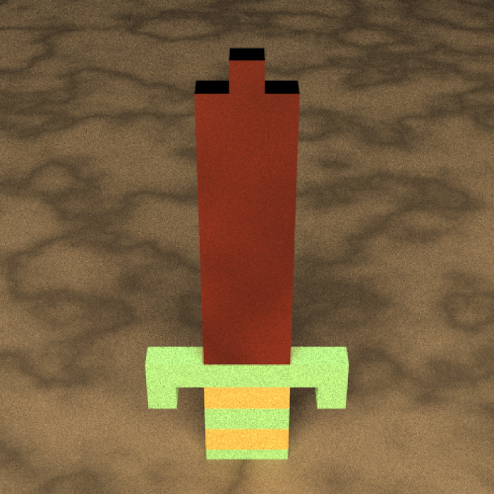
Now we add the R to the blade, using the same process but offseting it slightly towards the front of the blade.
scene2 = scene
rlogo = matrix(
c(1,1,1,0,
  1,0,0,1,
  1,1,1,0,
  1,0,1,0,
  1,0,0,1),
ncol = 4,byrow=TRUE)

material = metal(color="#be8d1b")

for(i in 1:ncol(rlogo)) {
  for(j in 1:nrow(rlogo)) {
    if(rlogo[j,i] != 0) {
      scene2 = add_object(scene2,cube(x=-0.4,y=8-j/2, z=-1.25+i/2,width=0.5, material=material))
    }
  }
}

render_scene(scene2,fov=30,width=500, height=500, samples=500,
             parallel=TRUE,lookfrom=c(-25,25,0),lookat = c(0,9,0))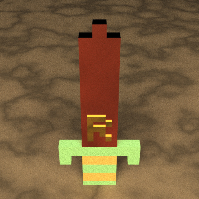
Finally, we rotate the camera around the sword and then turn all the images into a movie. To do this, we just specify the lookfrom coordinate to move in a circle centered around the lookat point. The odd subsetting I have included with the frame variable ensures you have a perfect loop, for extra Twitter points:
frames = 360

camerax=-25*cos(seq(0,360,length.out = frames+1)[-frames-1]*pi/180)
cameraz=25*sin(seq(0,360,length.out = frames+1)[-frames-1]*pi/180)

for(i in 1:frames) {
  render_scene(scene2, width=500, height=500, fov=35,
               lookfrom = c(camerax[i],25,cameraz[i]),
               lookat = c(0,9,0), samples = 1000, parallel = TRUE,
               filename=glue::glue("swordtest{i}"))
}

av::av_encode_video(glue::glue("swordtest{1:(frames-1)}.png"), framerate=60, output = "rswordfast.mp4")
file.remove(glue::glue("swordtestfast{1:(frames-1)}.png"))
Alternatively, you could just capture the plots directly using the av package and avoid saving any images to disk. I prefer to write the images to disk because you can then interrupt the process and not lose your progress, but for short animations this can be convenient:
av::av_capture_graphics(expr = {
  for(i in 1:frames) {
    render_scene(scene2, width=500, height=500, fov=35,
                 lookfrom = c(camerax[i], 25, cameraz[i]),
                 lookat = c(0,9,0),samples = 1000, parallel = TRUE)
  }
}, width=500,height=500, framerate = 60, output = "rsword2.mp4")It’s that easy! I hope you enjoyed this short introduction to the (very nascent) rayrender package. Support for more complex objects, materials, and rendering options are in the works. I’m going to push out a series of tutorials on more advanced topics as time goes on (implicit sampling, grouping of objects, animating). Be sure to sign up for my email list to learn more! You can also see the code and see more examples at the Github page below, as well as the package website:

Or just check out the examples and the documentation on the package’s website:
If you liked this post, be sure to sign up for my newsletter so you don’t miss future developments!