Slicing through Monterey Bay: Creating 3D Maps with Rayshader
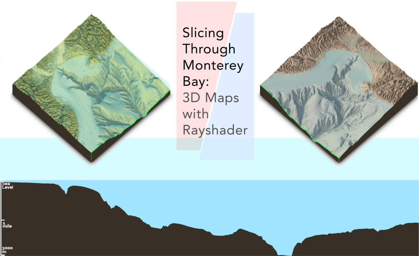
(See the bottom of the page for a description on how I generated the above figure–and read the rest of the article to see how to use rayshader and R to make beautiful 3D maps yourself.)
When I was a kid, my dad and I would occasionally take trips out on US-202 to Flemington, New Jersey to visit Northlandz ([ Video of Northlandz]) the world’s largest model railroad museum. As a kid who had a single functional railroad loop at home and a popsicle-stick town as its only stop–well, this place was something else. Hundreds of model trains driving on miles of tracks through detailed towns, bridges, gorgeous three-story hand-carved canyons–all miniturized so that you could take in an entire landscape in a single room. It was a 10-year-old boy’s nirvana, and it planted a seed of interest in scale models that has stuck with me–and shaped the latest features of rayshader.
Maps suffer from one major disadvantage when trying to represent a landscape: They are hopelessly flat.
I always enjoy a well-crafted, informative map, but maps suffer from one major disadvantage when trying to represent a landscape: They are hopelessly flat. You can add as many contours, raytraced/lambertian shadows, and spherical UV textures to try and convey the ebb and flow of the land–but those abstractions will only take our dumb primate brains so far. Being able to touch a landscape, walk around it, and examine it on a human scale conveys far more information than a carefully crafted contour ever could. I found a great example of this on a recent visit to Volcano National Park in Hawaii, featuring the topopgraphy and bathymetry of the Big Island in a 2-meter-wide weatherized scale model. It allowed you to drag your fingertips across the landscape and feel the volcanic craters and peaks; you could walk around the island and easily compare the slopes of Kona with the relative flatness of Hilo.
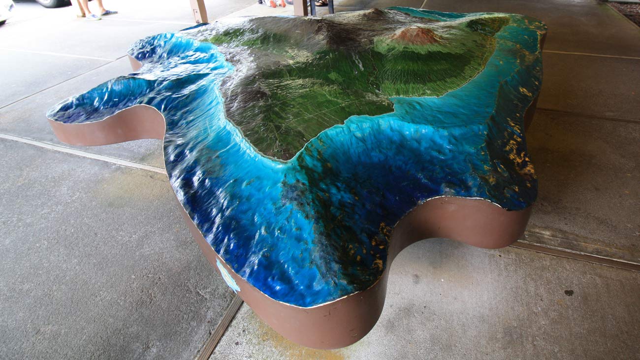
Figure 1: Bathymetric and topographic physical representation of the Big Island in Hawaii: also, good honeymoon destination.
Right before I released the last version of rayshader, I had a thought: I already have the elevation data and a surface texture, how hard would it be to combine the two in a 3D representation of the topography? I looked up the documentation for the rgl package and the answer was “not at all hard.” I wrote the function and generated a 3D surface with the texture, and I was blown away. The combination of the hillshaded texture and 3D representation in a dragable, interactive widget was about as close to a “tactile” experience you could have on a computer. And by setting the field of view to zero–which removes perspective and makes the scene isometric, simulating a model on your desk–it scratched that childhood itch of “miniturizing” the landscape.
elevation_matrix %>%
  sphere_shade() %>%
  add_shadow(ray_shade(elevation_matrix)) %>%
  add_shadow(ambient_shade(elevation_matrix)) %>%
  plot_3d()
detect_water feature. I have also adjusted the zscale argument to slightly exaggerate the heightmap.
While this floating surface was beautiful, it didn’t have the tangible “model” feel I was after: it still felt impossibly flat, regardless of the addition of a 3rd dimension. I didn’t want the map to look like a carefully crinkled sheet of paper; I wanted a 3D representation that looked like a paper weight, one that you could imagine setting on your work desk and occasionally picking up and examining when you needed a midday moment of introspection (i.e. when you are fidgeting). So I decided to build a base, and add a shadow:
elevation_matrix %>%
  sphere_shade(texture = "bw") %>%
  add_shadow(ray_shade(elevation_matrix)) %>%
  add_shadow(ambient_shade(elevation_matrix)) %>%
  add_water(detect_water(elevation_matrix),color = "unicorn") %>%
plot_3d(solid = TRUE, shadow = TRUE)This worked out pretty well, and succeeded in the “real physical object” effect that I was going after. And the actual base is completely customizable: you can change the color, transparency, height, line properties, shadow depth, and shadow width.
I didn’t want the map to look like a carefully crinkled sheet of paper; I wanted a 3D representation that looked like a paper weight.
Right after I developed that feature, @EarthObserved was livetweeting the talks at the Australian Marine Sciences Association Conference’s 2018 conference, and one particular tweet caught my eye. It was from a talk by Dr. Gary Greene about submarine canyon formation, and his presentation had a particular image:
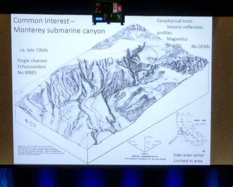
Figure 4: Tweet from Dr. Robbi Bishop-Taylor (@EarthObserved) on a talk about submarine canyon formation. Look familiar?
Almost identical to the map I had already generated–but with water! Inspired by this image (drafted decades before any computer generated software would make visualizing something like this easy), I decided to add a user-controlled water layer to the 3D maps produced by rayshader as well. The result:
elevation_matrix %>%
  sphere_shade(texture = "bw") %>%
  add_shadow(ray_shade(elevation_matrix)) %>%
  add_shadow(ambient_shade(elevation_matrix)) %>%
  plot_3d(solid = TRUE, shadow = TRUE, water = TRUE)
This also makes it extremely easy to perform analyses like the one I did in my previous post with Lake Mead: now you can quickly set the water level in the plot_3d call directly, rather than in the data itself. Setting the camera straight up phi = 90 and turning on an isometric view with fov = 0 gives you the standard GIS overhead view, and adjusting the water level is trivial.
waterdepthvalues = min(elevation_matrix)/2 - min(elevation_matrix)/2 * cos(seq(0,2*pi,length.out = 180))
thetavalues = 90 + 45 * cos(seq(0,2*pi,length.out = 180))

for(i in 1:180) {
  elevation_matrix %>%
    sphere_shade(texture = "imhof3") %>%
    add_shadow(ray_shade(elevation_matrix)) %>%
    add_shadow(ambient_shade(elevation_matrix)) %>%
    plot_3d(solid = TRUE, shadow = TRUE, water = TRUE,
            waterdepth = waterdepthvalues[i], watercolor = "imhof3", wateralpha = 0.8,
            waterlinecolor = "#ffffff", waterlinealpha = 0.5, waterlinewidth = 2,
            theta = thetavalues[i], phi = 45)
  rgl::snapshot3d(paste0("drain",i,".png"))
}
This ease of visualizing this layer makes performing analyses involving varying levels of water incredibly easy. Want to see how the beachfront will look if sea levels rose another 5 meters? Just get an elevation map of the surface, and set the water level in plot_3d to 5 meters. Want to see the worst case scenario of global warming melting the ice caps with a 75m in height? Change the 5 to 75. Want to see what your local beach looked like when sea levels were -125m lower at the peak of the ice age? Grab a bathymetric data set, and set the water level to -125. Easy.
Want to see what your local beach looked like when sea levels were -125m lower at the peak of the ice age? Grab a bathymetric data set, and set the water level to -125. Easy.
And with a fully realized 3D model of the surface and water, you can perform interesting visualizations like the one at the top of the page. The featured video of Monterey Bay at the top simply involved slicing a few rows of the elevation/depth matrix in a for loop, and then viewing that slice directly from the side. The same data was used to produce the rotating images, simply by moving the camera above and replacing those rows in the texture map (also produced programmatically by rayshader!) with green. In this whole process, there was only one piece of data that I needed to provide: an elevation matrix. Everything else is programmatically generated. And that has always been the main goal of rayshader: beautiful maps, derived directly from the elevation matrices.
for(i in 1:799) {
  montereybay_elevation[1:2+i,] %>%
    sphere_shade(texture = "imhof1",remove_edges = FALSE) %>%
    plot_3d(montereybay_elevation[1:2+i,],fov=0,theta=90,phi=0,
            solid = TRUE, background="white", solidlinecolor="grey50", solidcolor = "#373026",
            water=TRUE, waterdepth = 0,watercolor = "#88DDFF")
  rgl::snapshot3d(paste0("montbayslice_",i,".png"))
  rgl::rgl.close()
}
And that’s it for the latest set of features–next round will include depth of field for more “photographic” images, as well as support for using rayshader to easily build 3D ggplots. Below is the link to the github page:
rayshader on githubAnd if you want to see more cool stuff, follow me on Twitter and sign up for my newsletter for the latest updates on rayshader!