Roofs, Bevels, and Skeletons: Introducing the Raybevel Package

Intro

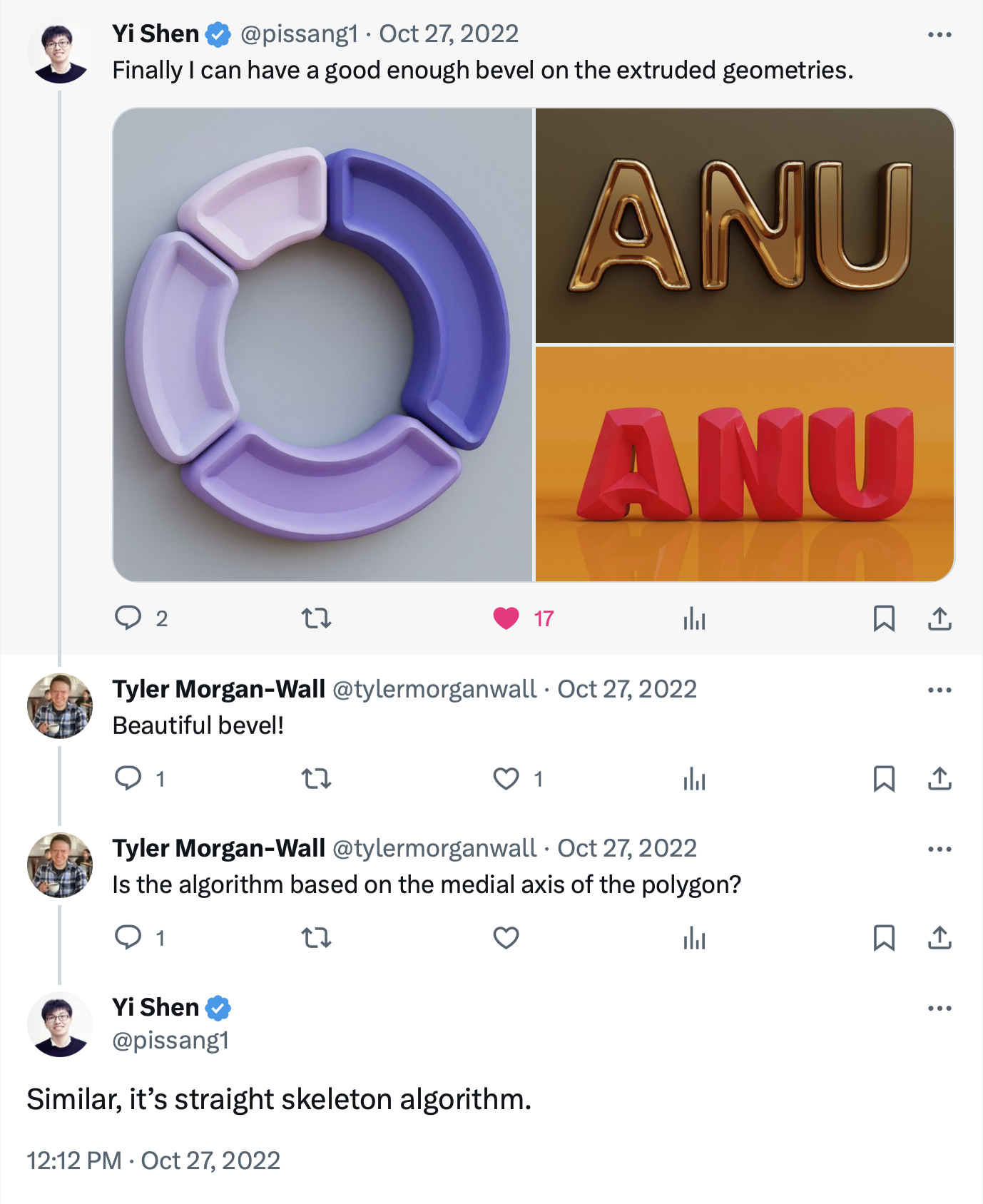
It all started with a tweet that caught my eye - a slick 3D rendering of beveled polygons by Yi Shen @pissang1.

Before a certain social media site went down the xitter

A couple things nerd-sniped me about this interaction: first, an algorithm I’ve never heard of? Check. One that can be used to create cool 3D meshes? Check again. And (after a few minutes of research) one that had no existing implementation in R? Check++.

The more I read, the more I realized that this would be a great new capability to add to R–and for more than just my rather niche interest in the 3D meshing and fancy beveling aspect. But first: what is a straight skeleton, and why is it useful?

Figure 1: The gold at the end of the rainbow (i.e. R package development process).

What is a straight skeleton?

#Load all libraries used in this plot
library(spData)
library(ggplot2)
library(sf)
library(av)
library(patchwork)
library(rnaturalearth)

#All the rayverse packages
library(rayrender)
library(rayvertex)
library(raybevel)

#Helper function: Center mesh in x/z coordinates
center_mesh_xz = function(x) {
  mesh_bbox = get_mesh_center(x)
  mesh_bbox[2] = 0
  translate_mesh(x,-mesh_bbox)
}

pennsylvania = spData::us_states[spData::us_states$NAME == "Pennsylvania",]
pa_skeleton = skeletonize(pennsylvania)
plot_skeleton(pa_skeleton)

1

Load the non-rayverse packages

2

Load the rayverse packages

3

Create a function used throughout the function to center meshes

4

Extract polygon of Pennsylvania from the us_states dataset

5

Skeletonize the polygon

6

Plot the skeleton (using raybevel, the package introduced in this post)

Figure 2: A straight skeleton of Pennsylvania. Why is this thing useful?

The straight skeleton of a polygon is the geometric object formed by tracing the vertices of a polygon as the edges propagate inwards. You can visualize this as a interior wavefront formed by all the edges of the polygon: vertices occur at places two edge’s wavefronts combine or split.

max_time = max(pa_skeleton$nodes$time)
pa_offsets = seq(0,max_time, length.out = 62)[c(-1,-62)]
for(i in 1:60) {
  ggplot() +
    plot_skeleton(pa_skeleton, return_layers = TRUE) +
    plot_offset_polygon(generate_offset_polygon(pa_skeleton,
                                                pa_offsets[i]), color = "green",
                        return_layers = TRUE) +
    theme_void() +
    theme(legend.position = "none",
          plot.background = element_rect(fill="white", color=NA)) +
    coord_fixed()
  ggsave(sprintf("pa_offset%i.png",i), width=8,height=4)
}
av::av_encode_video(input = sprintf("pa_offset%i.png",1:60), output = "wavefront.mp4")

1

Get the maximum internal distance out of the straight skeleton structure

2

Create offsets for these, except for the first and last values

3

Create frames of animations

4

Create animation mp4 file

Figure 3: Animating the internally propagating wavefront from the polygon edges. See the 3D version of this in Figure 6.

Straight Skeleton Applications

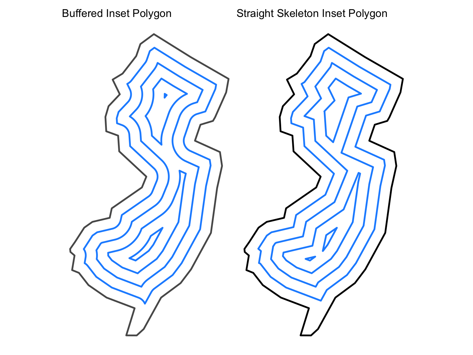
It’s useful for both 3D and 2D applications: one useful thing this algorithm can do create inset polygons that respect the topological and geometric properties of the original shape. These interior polygons preserve sharp corners, in contrast to st_buffer() which generates curved internal polygons (see Figure 4).

new_jersey = spData::us_states[spData::us_states$NAME == "New Jersey",] |>
  st_transform("EPSG:32111")
buffer_dist = seq(10000,40000,by=10000)
gglist = list()
for(i in seq_len(length(buffer_dist))) {
  new_jersey_buffered = st_buffer(new_jersey,-buffer_dist[i])
  gglist[[i]] = geom_sf(data = new_jersey_buffered, fill = NA,
                        linewidth = 1, color="dodgerblue")
}

buffer_inset = ggplot() +
  geom_sf(data = new_jersey, fill = NA, linewidth = 1) +
  gglist +
  theme_void() +
  labs(title = "Buffered Inset Polygon")

skeleton_inset = new_jersey |>
  skeletonize() |>
  generate_offset_polygon(offset = buffer_dist) |>
  plot_offset_polygon(plot_original_polygon = TRUE) +
  labs(title = "Straight Skeleton Inset Polygon")
buffer_inset + skeleton_inset

1

Extract and transform New Jersey polygon

2

Create buffer distances

3

Use {sf} to generate internal buffered polygons

4

Generate {sf}-based internal polygon ggplot

5

Generate {raybevel}-based straight skeleton internal polygon ggplot

6

Plot both with the patchwork package

Figure 4: {sf} buffered internal polygons vs straight skeleton inset polygons

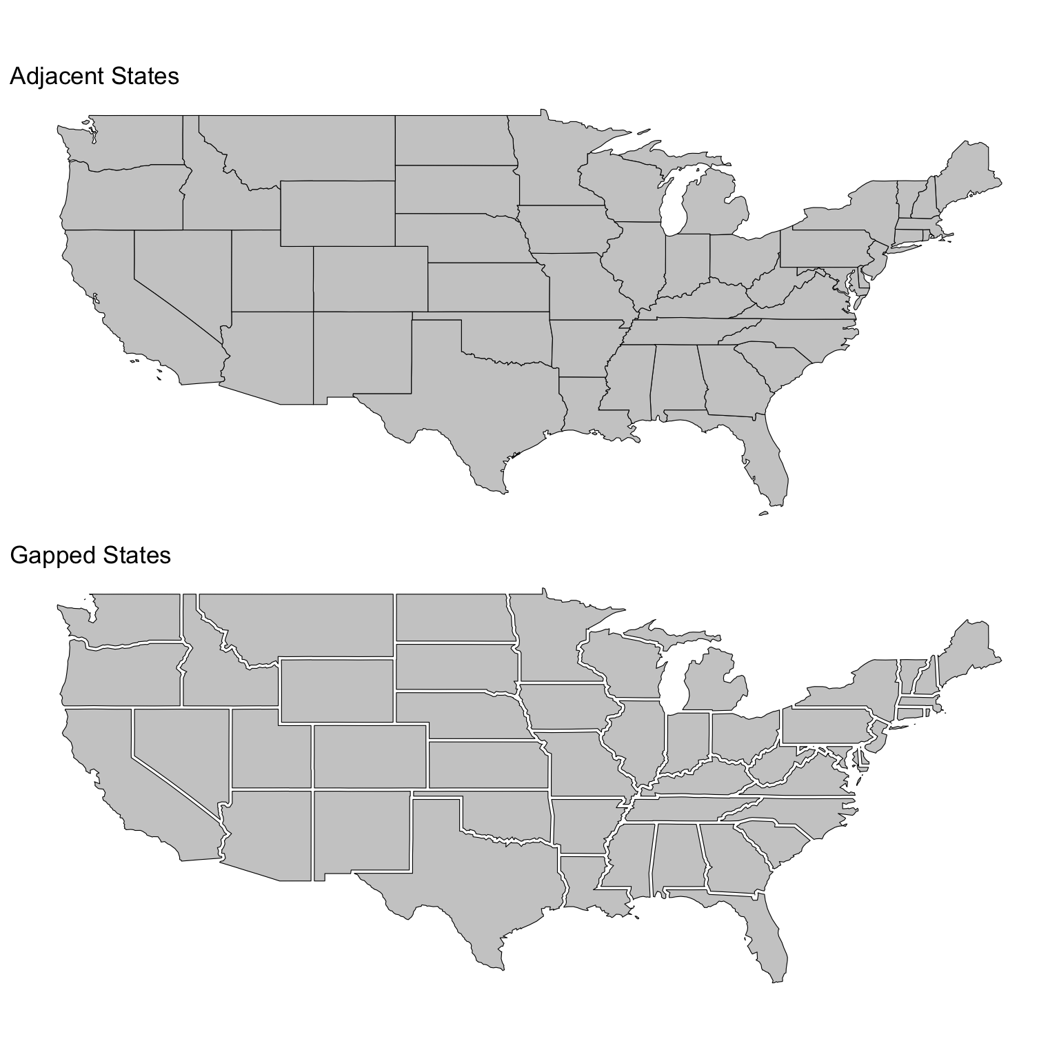
This is a much better option if you’ve ever resorted to negative buffers for manipulating polygons for aesthetic reasons: this package allows you to generate smaller polygons without introducing curves (for example, you can use this to create small gaps between directly-adjacent polygons without resorting to hacks with the border color).

us_plot = spData::us_states |>
  skeletonize() |>
  generate_offset_polygon(offset = 0) |>
  plot_offset_polygon(plot_original_polygon = FALSE,
                      color = "black", fill = "grey80",
                      linewidth = 0.2,
                      background = "white") +
  labs(title = "Adjacent States")

us_plot_gap = spData::us_states |>
  skeletonize() |>
  generate_offset_polygon(offset = 0.1) |>
  plot_offset_polygon(plot_original_polygon = FALSE,
                      color = "black", fill = "grey80",
                      linewidth = 0.2,
                      background = "white") +
  labs(title = "Gapped States")
us_plot / us_plot_gap

1

Generate the unchanged US state polygon ggplot

2

Generate the gapped US state polygon ggplot

3

Plot the two with {patchwork}

Figure 5: Adjacent state polygons versus gapped state polygons

This polygon shrinking process can also be represented continuously in 3D. Here’s where one of the really cool applications comes into play: 3D rooftops!

offset_pct = seq(0,1,length.out=61)[-1]
for(i in seq_len(length(offset_pct))) {
  pa_skeleton |>
    generate_beveled_polygon(base = TRUE,
                             bevel_offsets = generate_bevel(bevel_end = offset_pct[i],
                                                            angle = 45)) |>
    center_mesh_xz() |>
    raymesh_model(material = diffuse(color="purple")) |>
    add_object(xz_rect(xwidth=100,zwidth=100)) |>
    render_scene(lookfrom=c(-3,5,-3),fov=0,ortho_dimensions = c(5.5,5.5), lookat=c(-0.20, 0.67, -0.61),
                 filename = sprintf("generating_roof%i.png",i), width=800,height=800, samples=128,
                 preview=FALSE,
                 environment_light = "kiara_1_dawn_2k.hdr",rotate_env = i*6)
}

1

Generate offset percentages for animation

2

Render the image frames for the below animation.

Figure 6: This process represents the exact same 2D shrinking represented in Figure 3, but now in 3D.

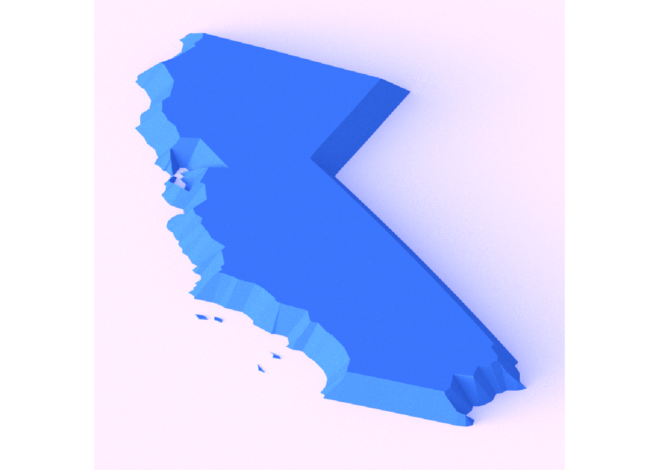
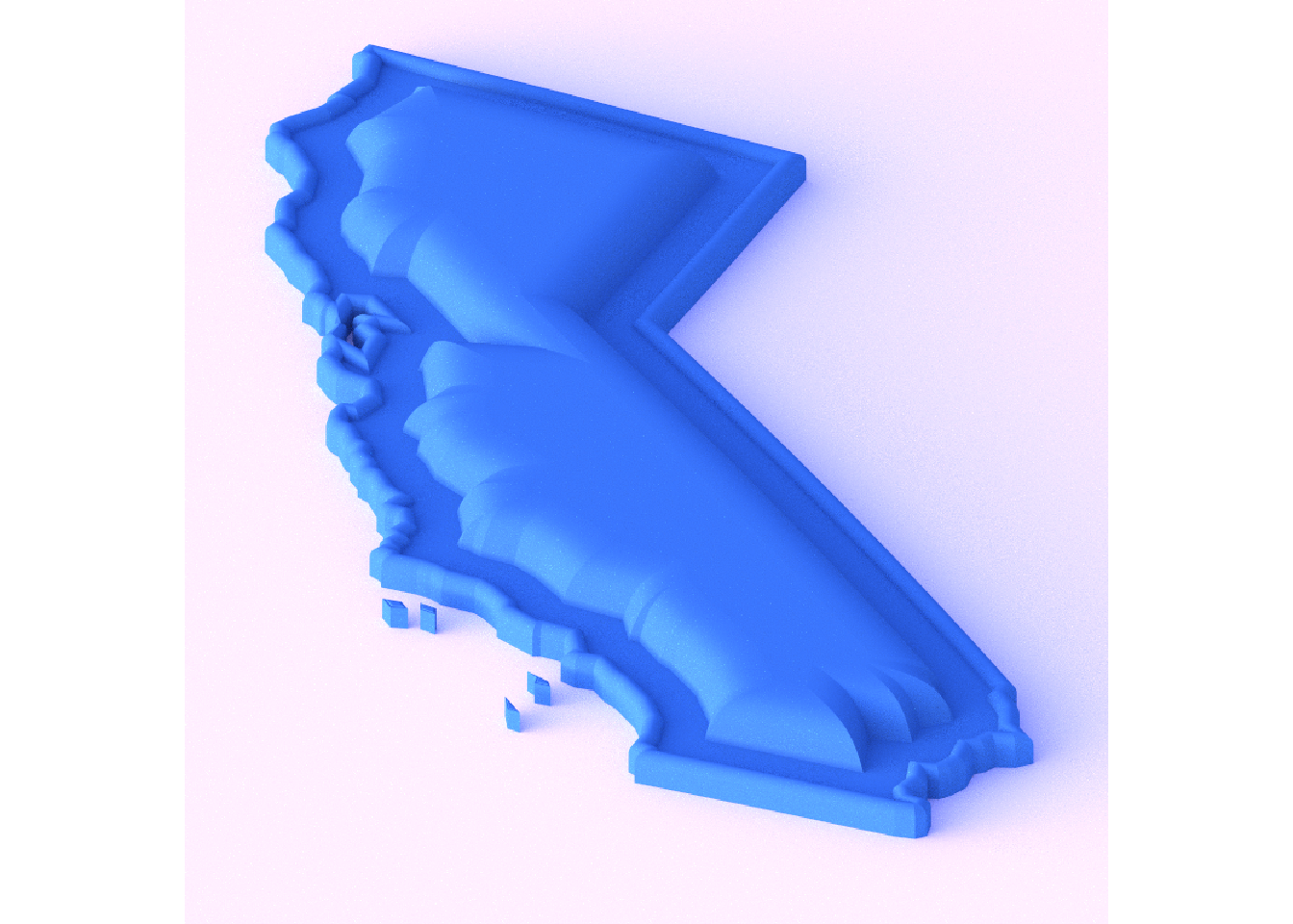
You can also use the straight skeleton to obtain internal polygon distance data and generate arbitrary bevels (the original goal of all this effort!).

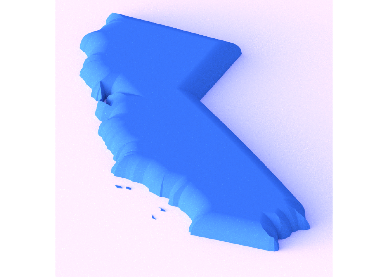
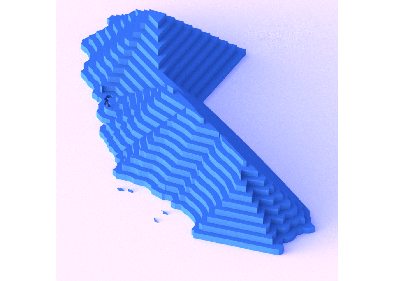
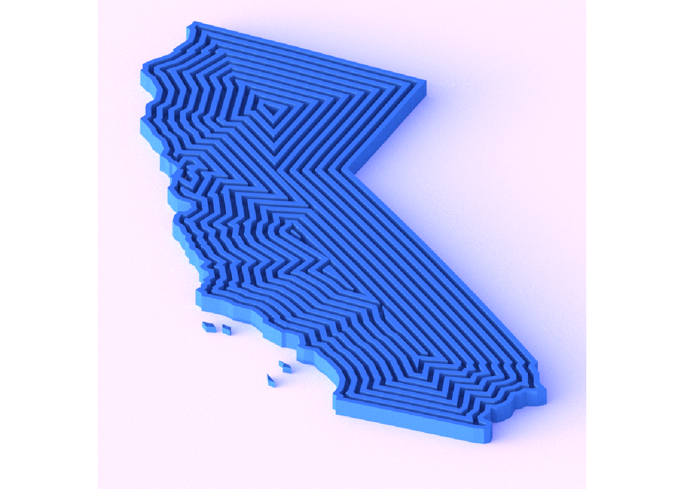
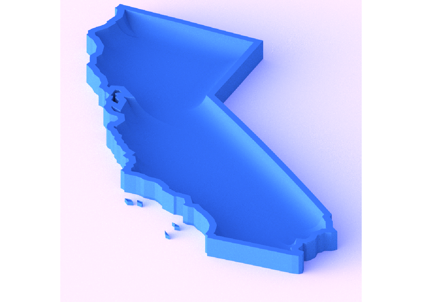
Figure 7: Inflating California like a balloon by applying an increasingly narrow smooth bevel.

There have also been other creative uses for the straight skeleton in GIS, such as road network simplification and estimating water drainage paths from height contours.

Developing the {raybevel} package

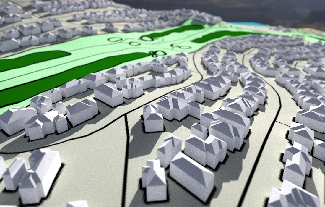
By itself, generating 3D rooftops was a strong enough motivator for me to add this capability to R and the rayverse: plain flat extruded polygons never had enough “character” to represent something as human and familiar as a house. It also serves as a data visualization cue: it’s nice to have a visual indicator (in this case, a sloping rooftop) that helps differentiate objects representing abstract 3D data from 3D buildings. But primarily, it would help provide a bit of humanity to visualizations of neighborhoods, which are plentiful in mapping.

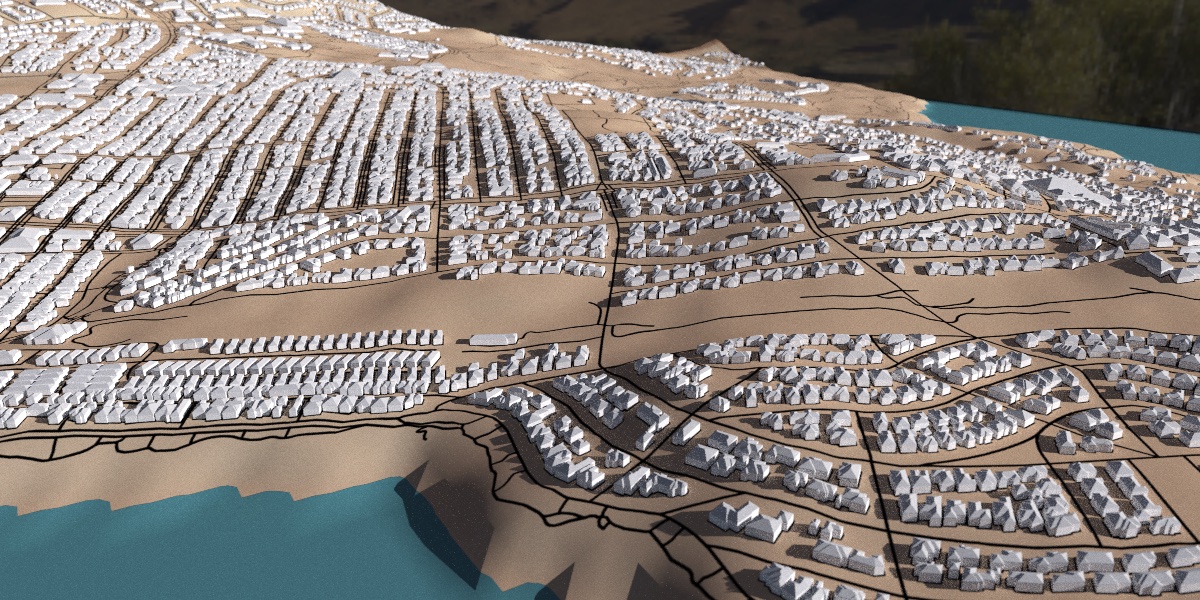
Figure 8: Comparing a neighborhood rendered with rooftops to one without.

Weighing the costs of complex dependencies

When I approach building a new package, I always start by doing some basic research: did anyone else already solve this in a header library I can wrap? Or is there an existing implementation in another language I can port to R? Straight skeleton generation is indeed available in the CGAL library, which has headers available via the RcppCGAL package. The Computational Geometry Algorithms Library (CGAL) is a robust, open-source software project that provides easy access to efficient and reliable geometric algorithms in the form of a C++ library. It encompasses a wide range of tools for computational geometry tasks, from basic geometric primitives to complex operations like mesh processing and geometry analysis. That power comes at a cost: the library is huge and complex, and due to its size requires a non-CRAN distribution method for the actual header files. And one thing I’ve learned over years of R package development is the danger of depending on another package for compiled code, particularly if it’s a non-standard installation process. The CRAN policies are fairly static, but the CRAN’s tooling is not: packages that are fine for years can suddenly have a two week deadline for removal looming over them because the latest version of GCC the CRAN uses is now throwing warnings.

Note

This just happened recently with the CRAN throwing -Wformat errors for the progress package, which propagated a 2-week removal warning to one of my packages–and by the time the progress package was uploaded and fixed, I only had a few days to issue my change! Additionally, the RcppCGAL package was taken down for several months this past year, and I worked with the maintainer to get it back up on the CRAN.

One of my choices as a solo R developer creating a universe of packages while also raising a kid, maintaining a house (e.g. surprise! your fridge is dead! hope you had no other weekend plans!), and working full time is to prioritize limiting surprise workloads with a deadline. It’s becoming more rare that I can drop everything and figure out a potentially complex workaround for a critical software dependency, so I try to only depend on my own universe of packages.

Don't trust the algorithm! Subscribe to my mailing list to be the first to learn about new blog posts.

* indicates required

Email Address *

/* real people should not fill this in and expect good things - do not remove this or risk form bot signups */

First attempts at a homegrown implementation

So I wanted to try to forgo the heavy CGAL dependency first, and luckily my research indicated that there were alternatives. Several people had seemed to have successfully created implementations of the Felkel and Obdržálek 1998 straight skeleton algorithm (polyskel and ladybug geometry). In particular, I saw that someone had adapted it for a plug-in for blender for creating 3D bpypolyskel and had done some testing showing robust performance (successful on 99.99% of OpenStreetMap building footprints). This algorithm was an attractive choice due to it’s relative simplicity–it only required implementing a circular linked-list data structure with some processing functions, and otherwise was a fairly small library. I decided to implement it in C++ for both speed and ease of translation, as working with circular reference-based data structures isn’t very natural in R. And after brushing up on my python and diving in, I finally had a working algorithm!

Figure 9: (Mostly) working custom straight skeleton implementation, drawing the straight skeleton of an undulating polygon.

Well, sort of. My data suggested the 99.99% performance number was a bit optimistic . My own numbers indicated that the algorithm failed significantly more frequently.

the nice results from the package testing on OSM buildings was likely due to most buildings having a fairly simple and similar structure

Figure 10: When nodes get close (see the center of the skeleton), the exact ordering of nodes within the straight skeleton graph is critical for correct meshes and internal polygons.

Here, the “correctness” of the straight skeleton structure depends on minute differences between nodes, and even with double precision I ran into issues.

Note

Part of the difficulty comes from the fact that the straight skeleton is inherently a non-local structure: tiny changes to the inputs can lead to wildly different skeleton configurations. Ensuring the resulting nodes are purely hierarchical (e.g. no loops or crossing links) is critical to the meshing process.

Poor results and lessons learned

It turns out the algorithm failed more frequently than I’d liked. I knew it wasn’t perfect going in, but the frequency of the failures (a rate closer to 1%-0.1% than 0.01% in my experience, and made worse as polygon complexity increased) made it pretty unusable for large-scale geographic visualizations. But it was not all wasted time–first of all, I got to brush up on some rusty python skills by translating an entire package with relatively complex data structures to C++! But more importantly, I had a much more intimate understanding of the straight skeleton structure, which was helpful when implementing 3D mesh/bevel generation. And with that understanding came the hard-earned knowledge that the straight skeleton structure was inherently computationally difficult to generate: it needs exact arithmetic for robustness, and thus the CGAL dependency is warranted. 🤷

Creating a CGAL-based straight skeleton package

Adopting CGAL wasn’t an insubstantial amount of work: significant amounts of infrastructure was needed to import R spatial/geometry data, calculate the skeleton, export out what I needed to R, and then actually do something interesting with the skeleton. CGAL outputs the straight skeleton structure as a half-edge data structure, which we will reduce to a simple directed graph. We’re then left with a simple directed graph with heights for each node. Additionally, the straight skeleton was only half the battle: I then needed to transform that data into 2D polygons and 3D meshes suitable for rendering in R. And not just simple 3D rooftops and simple 3D bevels: I wanted to support complex curved bevels, and thus needed a custom mesh generation algorithm.

Note

CGAL actually added the ability to generate meshes and simple 3D bevels halfway through 2023, about 4 months after I started working on this project: strange how these gaps in capability often seem to be noticed and solved in parallel! Thankfully, my implementation was more ambitious so my work was not wasted, but if that’s all I was after I could have just stopped here and written a lightweight wrapper around CGAL!

3D Meshing Algorithms

Roof generation was the easy part: let’s say we have a straight skeleton of a polygon and we want to generate a roof model. The roof height is already present by virtue of the straight skeleton providing a distance to each node from the edge: all we have to do is turn all the closed loops in the straight skeleton into polygons, and use the distance as the height of each vertex. This will give us a sloped roof (which you can scale to get different angles). The algorithm for this is relatively simple:

#Call internal raybevel function
polys = raybevel:::convert_ss_to_polygons(pa_skeleton)
ss = plot_skeleton(pa_skeleton, return_layers = TRUE)

ggpolys = lapply(polys, \(x) geom_polygon(data=pa_skeleton$nodes[x,2:3],
                                          aes(x=x,y=y), fill = "#ffaaaa",color = NA))

cntr = 1
for(i in seq_len(length(polys))) {
  poly = polys[[i]]
  poly = c(poly,poly[1])
  for(j in seq_len(length(poly))) {
    ggplot() +
      ggpolys[seq_len(i-1)] +
      ss +
      geom_path(data = pa_skeleton$nodes[poly[seq_len(j)],2:3],
                aes(x=x,y=y), color="purple", size=2) +
      theme_void() +
      theme(plot.background = element_rect(fill="white",color = NA)
            legend.position = "none") + 
      coord_fixed()
    ggsave(sprintf("demo_polygonization%i.png",cntr), width=8, heig
    cntr = cntr + 1
  }
  ggplot() +  
    ggpolys[seq_len(i)] +
    ss +
    theme_void() + 
    theme(plot.background = element_rect(fill="white",color = NA),
          legend.position = "none") + 
    coord_fixed()
  ggsave(sprintf("demo_polygonization%i.png",cntr), width=8, height
  cntr = cntr + 1
}

1

Call an internal {raybevel} function that converts a straight skeleton structure to polygons indices, pointing to vertices in the skeleton node structure

2

Generate the straight skeleton ggplot2 layers

3

Generate the straight skeleton polygon layers (one for each polygon)

4

Loop generating frames of the animation.

Figure 11: Visualizing the algorithm that turns the straight skeleton graph into polygons. Each one of these is then earcut to triangles.

3D Roof Meshes

Select a link not directly on the edge. Mark it as visited. Loop around the skeleton, taking the left-most turn at each node and recording the indices of the nodes you visit. When you return to the original vertex, those vertices form an interior polygon. Repeat for all non-edge links. When you’ve exhausted all links, de-duplicate the polygons by (in a copy of the list of indices) sorting each polygon’s indices and hashing the resulting vector. Earcut the polygons to triangulate the mesh. See an animated version of this algorithm above in Figure 11.

The straight skeleton structure defines the height of each vertex as the distance from the nearest edge, which means this algorithm works great for constant-slope rooftop generation. Let’s apply this algorithm to a few thousand houses and see how it looks in rayshader, using the new render_buildings() feature:

library(osmdata)
library(raster)

osm_bbox = c(-121.9472, 36.6019, -121.9179, 36.6385)

opq(osm_bbox) |>
  add_osm_feature("building") |>
  osmdata_sf() ->
osm_data

opq(osm_bbox) |>
  add_osm_feature("highway") |>
  osmdata_sf() ->
osm_road

building_polys = osm_data$osm_polygons
osm_dem = elevatr::get_elev_raster(building_polys, z = 11, clip = "bbox")
e = extent(building_polys)

osm_dem |>
  crop(e) |>
  extent() ->
new_e

osm_dem |>
  crop(e) |>
  raster_to_matrix() ->
osm_mat

osm_mat[osm_mat <= 1] = -2

osm_mat %>%
  rayimage::render_resized(mag=4) |>
  sphere_shade(texture = "desert") |>
  add_overlay(generate_polygon_overlay(building_polys, extent = new_e,
                                       heightmap = osm_mat,
                                       linewidth = 6,
                                       resolution_multiply = 50), rescale_original = TRUE) |>
  add_overlay(generate_line_overlay(osm_road$osm_lines, extent = new_e,
                                    heightmap = osm_mat,
                                    linewidth = 6,
                                    resolution_multiply = 50), rescale_original = TRUE) |>
  plot_3d(osm_mat, water = TRUE, windowsize = 800, watercolor = "dodgerblue",
          zscale = 10, theta=220, phi=22, zoom=0.45, fov=110,
          background = "pink")

render_buildings(building_polys,  flat_shading  = TRUE,
                 angle = 30 , heightmap = osm_mat,
                 material = "white", roof_material = "white",
                 extent = new_e, roof_height = 3, base_height = 0,
                 zscale=10)
render_highquality()

1

Load packages.

2

Specify the bounding box for the region we are pulling data from.

3

Get building polygon data road line data from OpenStreetMap

4

Get the actual extent the loaded building polygon data and use that to load elevation data using the elevatr package.

5

Crop DEM, but note that the cropped DEM will have an extent slightly different than what’s specified in e. Save that new extent to new_e.

6

Crop the DEM.

7

Visualize areas less than one meter as water (approximate tidal range)

8

Render the 3D rayshader scene

9

Generate and render the 3D building meshes from the polygon data

10

Render the scene with rayrender’s interactive pathtracer

Figure 12: Visualizing thousands of houses with rayshader’s new render_buildings() function.

3D Arbitrary Bevel Meshes

However, if we want to generate an arbitrary bevel instead of a simple roof, it gets a lot more complex: we need to insert new nodes at each distance defined in the bevel and link those horizontally nodes so they form constant height contours around the polygon. We then split the existing links at those bevel points and traverse the straight skeleton to link the new nodes together to form our contours. This latter step is trickier: as the interior polygon “shrinks” at higher interior distances, regions of the polygon can become disconnected from each other.

maryland = spData::us_states[spData::us_states$NAME == "Maryland",]
md_skeleton = skeletonize(maryland)
md_max_time = max(md_skeleton$nodes$time)
md_offsets = seq(0,md_max_time, length.out = 62)[c(-1,-62)]
for(i in 1:60) {
  ggplot() +
    plot_skeleton(md_skeleton, return_layers = TRUE,
                  size=0.5, arrow_size = 0.025) +
    plot_offset_polygon(generate_offset_polygon(md_skeleton,
                                                md_offsets[i]),
                        color = "dodgerblue",
                        return_layers = TRUE, linewidth = 1) +
    theme_void() +
    theme(legend.position = "none",
          plot.background = element_rect(fill="white", color=NA)) +
    coord_fixed()
  ggsave(sprintf("md_offset%i.png",i), width=8,height=4)
}
av_encode_video(input = sprintf("md_offset%i.png",1:60),
                output = "wavefront_md.mp4")

1

Extract the Maryland polygon

2

Skeletonize the polygon

3

Get the maximum internal distance out of the straight skeleton structure

4

Create offsets for these, except for the first and last values

5

Loop generating different offsets, showing the polygon breaking into several

6

Animate using {av}

Figure 13: You can see the polygon split multiple times into sub-polygons as the interior distance increases.

This complicates the meshing process significantly. There can be multiple polygons for a single interior polygon, and you need to be careful when traveling through the straight skeleton structure to only access areas that aren’t cut off yet. We ensure we do by scanning the entire straight skeleton network for local maxima: the peaks on the roof correspond to interior polygons that were topologically cut-off at one point.

md_skeleton |>
  generate_roof(base = TRUE) |>
  center_mesh_xz() |>
  raymesh_model(material = diffuse(color="purple")) |>
  add_object(xz_rect(xwidth=100,zwidth=100)) ->
rayscene

for(i in seq_len(180)) {
  render_scene(rayscene, lookfrom=c(7.07*sinpi(i*2/180),2,7.07*cospi(i*2/180))*2,
               fov=8,ortho_dimensions = c(5,5),
               filename = sprintf("md_peaks%i.png",i),
               width=800,height=300, samples=128,
               preview=FALSE,
               environment_light = "~/Desktop/hdr/kiara_1_dawn_2k.hdr")
}

1

Generate centered 3D rooftop mesh of Maryland

2

Render frames rotating around mesh.

Figure 14: Starting searches for offset polygons at the peaks (seen above in the 3D model) above the desired offset curve guarantees they will be found and ensures disconnected loops won’t be inadvertently connected.

We then always start our search from these maxima (when our contour is below that height) and only search the areas of the skeleton reachable from that point by always turning around when we insert a new node. This ensures we won’t connect nodes to other nodes that aren’t actually in the same interior polygon.

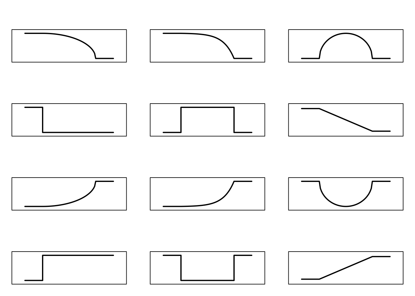
After modifying our straight skeleton structure with new links, we just apply the same polygonization algorithm as in the simple rooftop case! To apply our custom bevel, we just take each node’s distance from the edge and interpolate its height to the height specified in the input bevel. This transforms the interior of our polygon into any 3D profile we want! Here’s some that are build into {raybevel}:

par(mfrow = c(4, 3), mai = c(0.2, 0.2, 0.5, 0.2))
types = rep(c("circular", "exp", "bump", "step", "block", "angled"),2)
reverses = c(rep(FALSE,6),rep(TRUE,6))
for(i in seq_len(length(types))) {
  coords = generate_bevel(types[i], 0.2, 0.8, 1, flip = TRUE,
                          angle = 45, reverse = reverses[i], plot_bevel = TRUE)
}

1

Set up base R plot

2

Visualize each of the built-in bevels in raybevel

3

Also include the reversed bevels

4

Plot them all

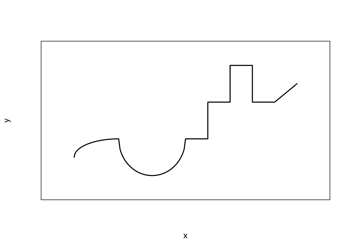
raybevel also includes helper functions to help you create complex bevels, although you can also just manually pass a list with x/y coordinates with your own bevel.

complex_coords = generate_complex_bevel(
  bevel_type  = c("circular", "bump", "step", "block", "angled"),
  bevel_start = c(0,   0.2, 0.6, 0.7, 0.9),
  bevel_end   = c(0.2, 0.5, 0.7, 0.8, 1.0),
  segment_height  = c(0.1, 0.2, 0.2, 0.2, 0.4),
  angle = 45,
  curve_points = c(50, 50, 50, 1, 1),
  reverse = c(FALSE, TRUE, FALSE, FALSE, FALSE),
  plot_bevel = TRUE
)

Examples of visualizations made with {raybevel}

What visual effects we do with this algorithm? Lots! We can add nice simple bevels to polygons:

ca_skeleton =  skeletonize(spData::us_states[spData::us_states$NAME == "California",])
ca_skeleton |>
  generate_beveled_polygon(base = TRUE,
                           bevel_offsets = generate_bevel(angle=45)) |>
  center_mesh_xz() |>
  raymesh_model(material = diffuse(color="dodgerblue4")) |>
    add_object(xz_rect(xwidth=100,zwidth=100)) |>
    render_scene(lookfrom=c(-2.39, 3.50, -5.00),fov=0,ortho_dimensions = c(8,8),
                 width=800,height=800, samples=128, preview=FALSE,
                 environment_light = "~/Desktop/hdr/kiara_1_dawn_2k.hdr")

1

Generate straight skeleton of California

2

Render 3D beveled California mesh using rayrender

Figure 15: California with a chamfered edge

Create smooth edges:

smooth_bevel = generate_bevel("circular",
                              bevel_end = 0.3, max_height = 0.3)

ca_skeleton |>
  generate_beveled_polygon(base = TRUE,
                           bevel_offsets = smooth_bevel) |>
  center_mesh_xz() |>
  raymesh_model(material = diffuse(color="dodgerblue4")) |>
    add_object(xz_rect(xwidth=100,zwidth=100)) |>
    render_scene(lookfrom=c(-2.39, 3.50, -5.00),fov=0,ortho_dimensions = c(8,8),
                 width=800,height=800, samples=128, preview=FALSE,
                 environment_light = "~/Desktop/hdr/kiara_1_dawn_2k.hdr")

1

Generate a bevel with {raybevel}’s generate_bevel() function.

2

Render 3D beveled California mesh using rayrender

Figure 16: California with a smooth, beveled corner

Or complex transformations like turn a polygon into a ziggarat:

ziggarat_bevel = generate_complex_bevel("step",
                                        segment_height = 0.1,
                                        bevel_start = seq(0,0.9,by=0.1),
                                        bevel_end = seq(0.1,1,by=0.1))

ca_skeleton |>
  generate_beveled_polygon(base = TRUE,
                           bevel_offsets = ziggarat_bevel) |>
  center_mesh_xz() |>
  raymesh_model(material = diffuse(color="dodgerblue4")) |>
    add_object(xz_rect(xwidth=100,zwidth=100)) |>
    render_scene(lookfrom=c(-2.39, 3.50, -5.00),fov=0,ortho_dimensions = c(8,8),
                 width=800,height=800, samples=128, preview=FALSE,
                 environment_light = "~/Desktop/hdr/kiara_1_dawn_2k.hdr")

1

Generate a complex, multi-segment bevel with {raybevel}’s generate_complex_bevel() function.

2

Render 3D beveled California mesh using rayrender

Figure 17: California as a ziggarat

Or use negative bevels to form a labyrinth-like pattern:

labyrinth_bevel = generate_complex_bevel("step",
                                         segment_height = 0.1,
                                         bevel_start = seq(0,0.95,by=0.05),
                                         bevel_end = seq(0.05,1,by=0.05),
                                         reverse = c(FALSE, TRUE))

ca_skeleton |>
  generate_beveled_polygon(base = TRUE,
                           offset=0.1,
                           bevel_offsets = labyrinth_bevel) |>
  center_mesh_xz() |>
  raymesh_model(material = diffuse(color="dodgerblue4")) |>
    add_object(xz_rect(xwidth=100,zwidth=100)) |>
    render_scene(lookfrom=c(-2.39, 3.50, -5.00),fov=0,ortho_dimensions = c(8,8),
                 width=800,height=800, samples=128, preview=FALSE,
                 environment_light = "~/Desktop/hdr/kiara_1_dawn_2k.hdr")

1

Generate a labyrinth-style bevel by reversing the bevel every other segment

2

Render 3D beveled California mesh using rayrender

Figure 18: California with a maze-like interior

Or a create a California bowl:

labyrinth_bowl = generate_complex_bevel(c("step","exp"),
                                         segment_height = 0.25,
                                         bevel_start = c(0,0.1),
                                         bevel_end = c(0.1,0.5),
                                         reverse = c(FALSE, TRUE))

ca_skeleton |>
  generate_beveled_polygon(base = TRUE,
                           offset=0.1,
                           bevel_offsets = labyrinth_bowl) |>
  center_mesh_xz() |>
  raymesh_model(material = diffuse(color="dodgerblue4")) |>
    add_object(xz_rect(xwidth=100,zwidth=100)) |>
    render_scene(lookfrom=c(-2.39, 3.50, -5.00),fov=0,ortho_dimensions = c(8,8),
                 width=800,height=800, samples=128, preview=FALSE,
                 environment_light = "~/Desktop/hdr/kiara_1_dawn_2k.hdr")

1

Generate a bowl by reversing the second bevel after stepping up some distance

2

Render 3D beveled California mesh using rayrender

Figure 19: California as a bowl

Or even more complex things, like a bump around the edges with a bigger interior bevel (this is the basis behind the animation shown in Figure 1):

bevel_bump = generate_complex_bevel(c("bump", "exp"),
                               bevel_start = c(0,0.3),
                               bevel_end = c(0.1,0.6),
                               segment_height = c(0.05,0.2))

ca_skeleton |>
  generate_beveled_polygon(base = TRUE,
                           bevel_offsets = bevel_bump,
                           offset = 0.2) |>
  center_mesh_xz() |>
  raymesh_model(material = diffuse(color="dodgerblue4")) |>
    add_object(xz_rect(xwidth=100,zwidth=100)) |>
    render_scene(lookfrom=c(-2.39, 3.50, -5.00),fov=0,ortho_dimensions = c(8,8),
                 width=800,height=800, samples=128, preview=FALSE,
                 environment_light = "~/Desktop/hdr/kiara_1_dawn_2k.hdr")

1

Generate a multi-segment bevel by specifying multiple bevel types

2

Render 3D beveled California mesh using rayrender

Figure 20: California with a bumped edge and raised interior

We can even just specify our own bevels directly with mathematical functions:

ca_skeleton |> 
  generate_beveled_polygon(base = TRUE, 
                           bevel_offsets = seq(0,3,by=0.1)/3,
                           bevel_heights = abs(exp(seq(0,3,by=0.1)))/20 +
                             sinpi(seq(0,3,by=0.1))/10,
                           offset=0.2) |> 
  center_mesh_xz() |>
  raymesh_model(material = diffuse(color="dodgerblue4")) |>
    add_object(xz_rect(xwidth=100,zwidth=100)) |>
    render_scene(lookfrom=c(-2.39, 3.50, -5.00),fov=0,ortho_dimensions = c(8,8),
                 width=800,height=800, samples=128, preview=FALSE,
                 environment_light = "~/Desktop/hdr/kiara_1_dawn_2k.hdr")

1

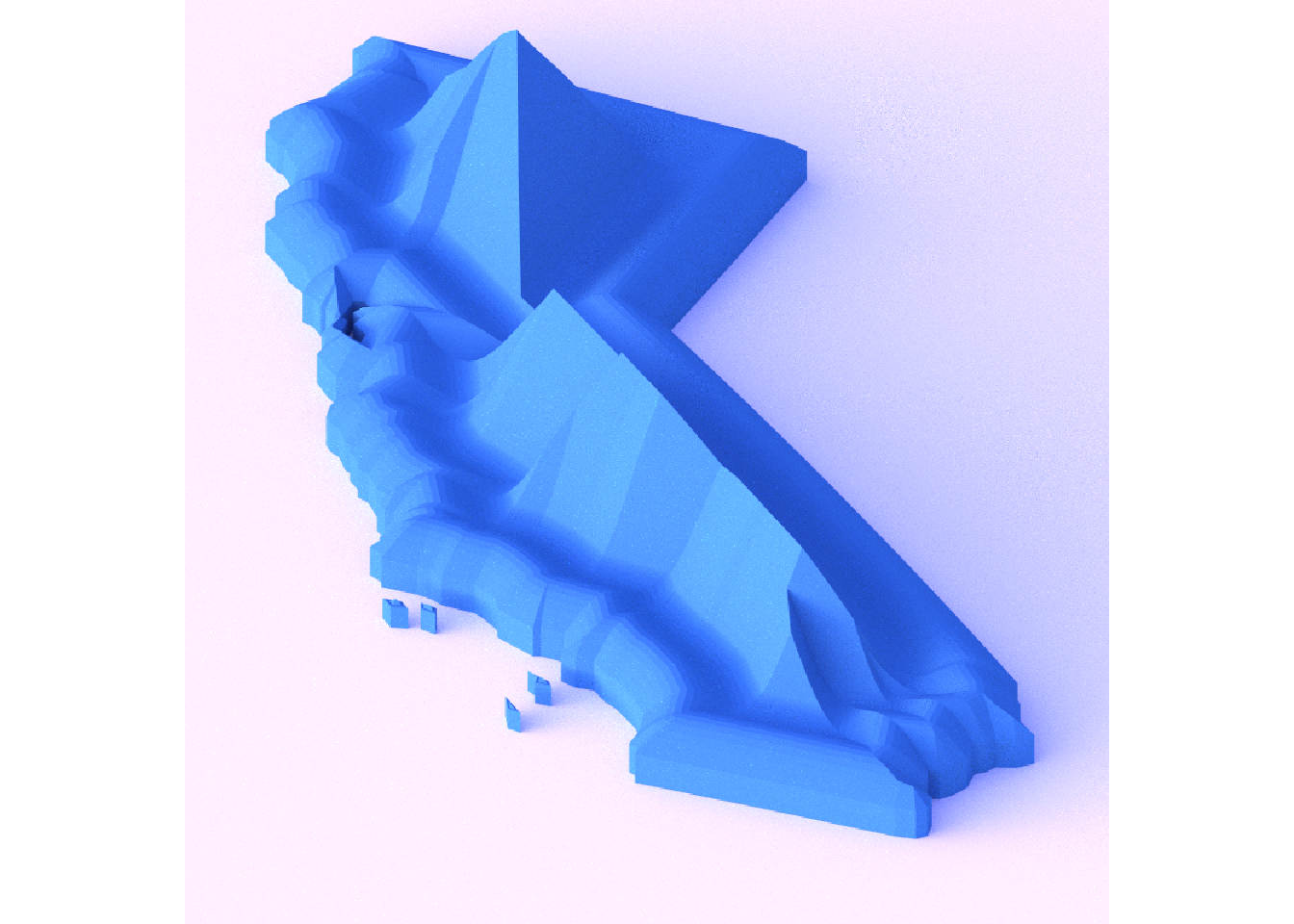
Generate the bevel manually using mathematical functions

2

Render 3D beveled California mesh using rayrender

Figure 21: California with a custom bevel defined by math functions

Or crazy things like make SVG fonts into double-sided bubble letters by applying a circular edge contour:

Figure 22: This did require writing an entirely new package for importing SVG as polygons, but that’s a yak that’s not yet completely shorn!

I’ve packaged up all these functions into the new package raybevel: simply input polygons or sf objects and transform them to 3D, or create 2D inset polygons! I’ve used it throughout this post, I’ve also included interfaces built-in to rayshader (render_buildings()) and render_beveled_polygons()).

Creating the {raybevel} hexlogo

Finally, it’s my personal philosophy that any R package focused on making cool and interesting visualizations should use itself to generate it’s package hexlogo. So I pulled up Inkscape and started working on a logo…

Figure 23: Base hexlogo design

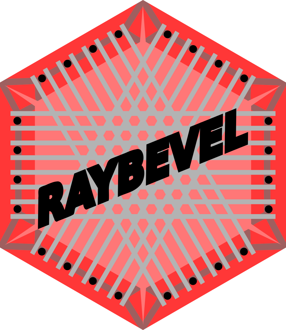
I decided I wanted to have bolts added to the edge plates on the center lines of the polygons, but there was no way in Inkscape to do that easily. If only there was some way to get the mid-line of the polygon! Oh wait, didn’t I just write a package for generating straight skeletons? One round trip to R/raybevel and back to SVG later…

Figure 24: Finding the center lines of the polygons by computing the straight skeleton in R, exporting it back to SVG, and overlaying it in Inkscape

With bevels applied to each polygon along with a metallic material and knurling added as a bump map, we then end up with this sparkling new pathtraced hexlogo:

Figure 25: Final hexlogo render

Awesome! The package is complete. Now R users can make 2D inset polygons, beautiful beveled 3D shapes, and slick 3D rooftops. Happy New Year!

Links

Raybevel Github

Raybevel Site

Rayshader Github

Rayshader Site