How to: Download and Animate Polar Ice Data in R with Rayrender
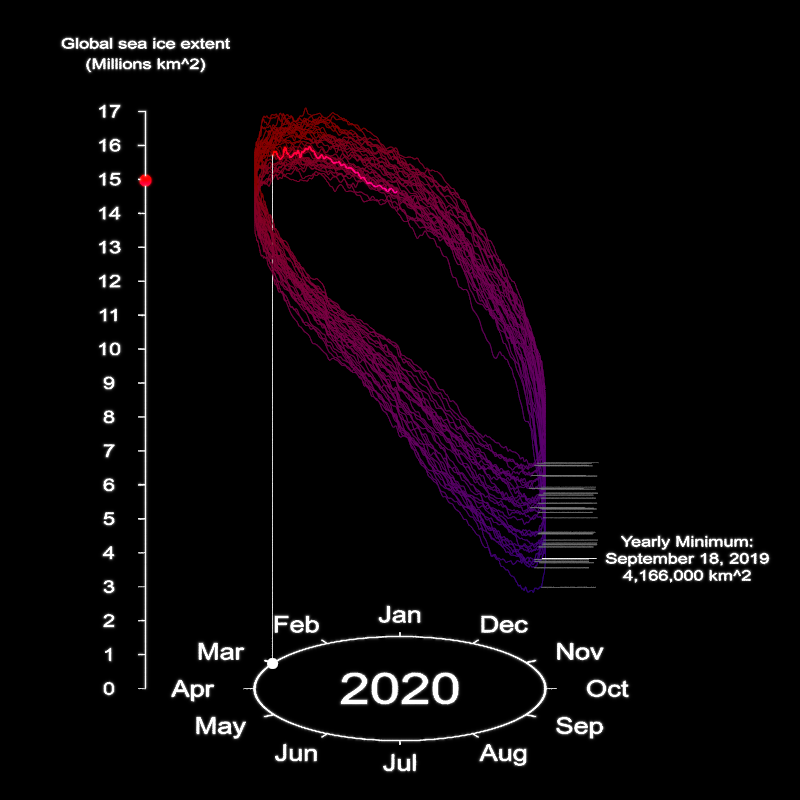
This post will serve as a guide on making the above visualization entirely in R (using rayrender), directly from the data source! I wanted to create an example of how your could create a complex, multi-faceted 3D visualization, entirely in R. I’ve provided all the code so you can generate the visualization from scratch—this can hopefully provide you with several strategies and workflows so you can create beautiful 3D visualizations in R yourself.
We need two sources of data for this visualization: the sea ice extent polygons for both the arctic and antarctic along with the daily sea ice global area. We’ll first start with loading the monthly sea ice extent polygon data from the National Snow and Ice Data Center (NSIDC). NSIDC hosts the data on an FTP server, so we’ll pull the list of files and then download each shapefile individually.
First we download the Arctic data using RCurl:
require(RCurl)

ice_dates = c("01_Jan", "02_Feb", "03_Mar", "04_Apr", "05_May", "06_Jun",
  "07_Jul", "08_Aug", "09_Sep", "10_Oct", "11_Nov", "12_Dec")

#Arctic
sea_url = "ftp://sidads.colorado.edu/DATASETS/NOAA/G02135/north/monthly/shapefiles/shp_extent/"

#Load all years of data, for each month
for(i in 1:12) {
  sea_url_single = glue::glue("{sea_url}{ice_dates[i]}/")
  filenames = getURL(sea_url_single, ftp.use.epsv = FALSE, dirlistonly = TRUE)
  filenames = strsplit(filenames, "\n")
  filenames = unlist(filenames)
  filenames = filenames[!filenames %in% c(".","..")]
  for (filename in filenames) {
    download.file(paste(sea_url_single, filename, sep = ""),
                  paste(getwd(), "/", filename,sep = ""))
  }
}
And then run the same code, but now for the Antarctic data:
#Antarctic

sea_url_south = "ftp://sidads.colorado.edu/DATASETS/NOAA/G02135/south/monthly/shapefiles/shp_extent/"
sea_url_single = glue::glue("{sea_url_south}{ice_dates[1]}/")

#Load all years of data, for each month

for(i in 1:12) {
  sea_url_single = glue::glue("{sea_url_south}{ice_dates[i]}/")
  filenames = getURL(sea_url_single, ftp.use.epsv = FALSE, dirlistonly = TRUE)
  filenames = strsplit(filenames, "\n")
  filenames = unlist(filenames)
  filenames = filenames[!filenames %in% c(".","..")]
  for (filename in filenames) {
    download.file(paste(sea_url_single, filename, sep = ""),
                  paste(getwd(), "/", filename, sep = ""))
  }
}
Now, we’re going to load the polygon data into R, and then plot it in 3D over a world map. This requires a few moving parts: the sf package to read in the data, the anglr/silicate/quadmesh packages to project the polygons onto a 3D sphere, and then the rgl package to write the 3D polygon to an OBJ file (that’s then imported by rayrender).
Let’s first load some of our packages:
library(sf)
library(maptools)
library(raster)
library(anglr)
library(silicate)
library(quadmesh)
library(rgl)
library(rayrender)
We’re going to generate two separate visualizations and combine them to create the visualization above. First we’ll generate the polar world map that shows the actual polar ice caps on the right. We’ll render an image for each year and month: when the 3D line graph on the left passes through that month and year, we’ll display the corresponding polar polygon data. This way we only have to generate about 360 (12 months * 30 years) images for the right half of the visualization, versus the full 11924 frames for the left.
Our data is given in monthly intervals: let’s write a function that will take the month and year we want and write our two 3D models to the current directory. This function unzips the polygon to a temporary directory, reads the polygon in using sf, generates a Delaunay triangulation (with a maximum triangle size, which preserves interior points and thus captures the curvature of the earth), creates a mesh out of it, projects that mesh onto a sphere, and then writes the mesh to an OBJ file. It does this for both the arctic (arctic.obj) and antarctic (antarctic.obj).
generate_sea_obj = function(yearval, mon_val) {
  #South
  temp_ice_dir = tempdir()
  sea_ice_temp = unzip(sprintf("extent_S_%d%02d_polygon_v3.0.zip",yearval,mon_val),
                       exdir = temp_ice_dir)
  temp_address = sprintf("%s/extent_S_%d%02d_polygon_v3.0.shp",temp_ice_dir,yearval,mon_val)
  ice_layer = sf::st_read(temp_address)

  ice_layer_mesh  =sf::st_read(temp_address) %>%
    DEL(max_area = 500000000) %>%
    as.mesh3d(smooth=TRUE, color="red")
  ice_layer_mesh$vb[1:3,] = t(llh2xyz(
    reproj::reproj(t(ice_layer_mesh$vb[1:3,]),
                   source = crs(ice_layer),
                   target="+proj=longlat +datum=WGS84")))
  plot3d(ice_layer_mesh,box=FALSE,axes=FALSE)
  Sys.sleep(0.2)

  rgl::aspect3d("iso")
  Sys.sleep(0.2)
  rgl::writeOBJ("antarctic.obj")
  Sys.sleep(0.2)

  rgl::rgl.clear()
  #North
  sea_ice_temp = unzip(sprintf("extent_N_%d%02d_polygon_v3.0.zip", yearval,mon_val),
                       exdir = temp_ice_dir)
  temp_address = sprintf("%s/extent_N_%d%02d_polygon_v3.0.shp",temp_ice_dir,yearval,mon_val)
  ice_layer  =sf::st_read(temp_address)

  ice_layer_mesh  =sf::st_read(temp_address) %>%
    DEL(max_area = 500000000) %>%
    as.mesh3d(smooth=TRUE, color="red")
  ice_layer_mesh$vb[1:3,] = t(llh2xyz(
    reproj::reproj(t(ice_layer_mesh$vb[1:3,]),
                   source = crs(ice_layer),
                   target="+proj=longlat +datum=WGS84")))
  plot3d(ice_layer_mesh,box=FALSE,axes=FALSE)
  Sys.sleep(0.2)

  rgl::aspect3d("iso")
  Sys.sleep(0.2)

  rgl::writeOBJ("arctic.obj")
  Sys.sleep(0.2)

  rgl::rgl.clear()
}
Now let’s generate the 3D pathtraced polar map on the right. We’ll generate our monthly OBJ file using generate_sea_obj(), place it on top of a sphere with a world map superimposed, load it into a virtual photo studio generated using generate_studio(), and light up the scene with a single sphere light. The data starts in February 1988 and ends in September of 2020, so we’ll skip the first month in 1988 and break out of the loop when it hits October 2020.
yearvals = 1988:2020
mon_vals = 1:12

for(yearval in yearvals) {
  for(mon_val in mon_vals) {
    if(yearval == 1988 && mon_val == 1) {
      next
    }
    if(yearval == 2020 && mon_val == 10) {
      break
    }
    generate_sea_obj(yearval,mon_val)
    generate_studio() %>%
      add_object(sphere(x=1,radius=1,angle=c(-90,0,0),material = glossy(gloss=0.2,
        image_texture = "earth.png"))) %>%
      add_object(sphere(x=-1,radius=1,angle=c(-90,180,0),material = glossy(gloss=0.2,
        image_texture = "earth.png"))) %>%
      add_object(obj_model(x=1,"arctic.obj", z=0.0001,scale_obj = 1/6378100 ,
                           material=glossy(),angle=c(0,0,0))) %>%
      add_object(obj_model(x=-1,"antarctic.obj", z=0.0001,scale_obj = 1/6378100 ,
                           material=glossy(), angle=c(0,180,0))) %>%
      add_object(sphere(y=5,z=5,radius=2,material=light(intensity =10))) %>%
      render_scene(width=800,height=800,aperture=0, fov=25,sample_method = "stratified",
                   samples=500, clamp_value=10, lookfrom=c(0,1,10),
                   filename=glue::glue("seaice_{yearval}_{mon_val}.png"))
  }
}
Done! Now, let’s generate the line plot on the left. This is a bit more involved :)
First, we must load and process the daily sea ice data. I’ve included a cleaned up version of the dataset here. We’ll use dplyr and reshape2 to take clean and transform the data into the format we require to plot it in 3D. Specifically, we need to map the date to a point around a circle. Since we’re working with dates, we’ll take advantage of the great lubridate package.
library(reshape2)
library(dplyr)
library(lubridate)

sea_ice <- read.csv("sea_ice.csv")
gt::gt(head(sea_ice))| Month | Day | X1978 | X1979 | X1980 | X1981 | X1982 | X1983 | X1984 | X1985 | X1986 | X1987 | X1988 | X1989 | X1990 | X1991 | X1992 | X1993 | X1994 | X1995 | X1996 | X1997 | X1998 | X1999 | X2000 | X2001 | X2002 | X2003 | X2004 | X2005 | X2006 | X2007 | X2008 | X2009 | X2010 | X2011 | X2012 | X2013 | X2014 | X2015 | X2016 | X2017 | X2018 | X2019 | X2020 |
|---|---|---|---|---|---|---|---|---|---|---|---|---|---|---|---|---|---|---|---|---|---|---|---|---|---|---|---|---|---|---|---|---|---|---|---|---|---|---|---|---|---|---|---|---|
| January | 1 | NA | NA | 14.200 | 14.256 | NA | 14.253 | NA | NA | 14.036 | NA | NA | 14.261 | 14.319 | 13.634 | 14.069 | 14.035 | 14.095 | 14.145 | 13.804 | 13.657 | 14.025 | 13.823 | 13.442 | 13.479 | 13.590 | 13.647 | 13.502 | 13.160 | 13.160 | 13.110 | 13.206 | 13.189 | 13.205 | 12.896 | 13.353 | 12.959 | 13.011 | 13.073 | 12.721 | 12.643 | 12.484 | 12.934 | 13.102 |
| January | 2 | NA | 14.997 | NA | NA | 14.479 | NA | 14.103 | 14.045 | NA | 14.305 | NA | 14.313 | 14.384 | 13.831 | 14.092 | 14.141 | 14.110 | 14.258 | 13.818 | 13.801 | 14.097 | 13.886 | 13.539 | 13.385 | 13.628 | 13.698 | 13.538 | 13.163 | 13.210 | 13.207 | 13.164 | 13.180 | 13.232 | 12.915 | 13.421 | 12.961 | 13.103 | 13.125 | 12.806 | 12.644 | 12.600 | 12.992 | 13.075 |
| January | 3 | NA | NA | 14.302 | 14.456 | NA | 14.306 | NA | NA | 14.292 | NA | NA | 14.402 | 14.283 | 13.847 | 14.141 | 14.250 | 14.042 | 14.335 | 13.786 | 13.837 | 14.262 | 13.884 | 13.630 | 13.418 | 13.598 | 13.876 | 13.502 | 13.293 | 13.267 | 13.182 | 13.190 | 13.267 | 13.254 | 12.926 | 13.379 | 13.012 | 13.116 | 13.112 | 12.790 | 12.713 | 12.634 | 12.980 | 13.176 |
| January | 4 | NA | 14.922 | NA | NA | 14.642 | NA | 14.237 | 14.240 | NA | 14.417 | NA | 14.417 | 14.321 | 13.858 | 14.072 | 14.255 | 14.168 | 14.288 | 13.791 | 13.864 | 14.277 | 13.913 | 13.657 | 13.510 | 13.623 | 13.925 | 13.590 | 13.313 | 13.307 | 13.252 | 13.275 | 13.286 | 13.236 | 13.051 | 13.414 | 13.045 | 13.219 | 13.051 | 12.829 | 12.954 | 12.724 | 13.045 | 13.187 |
| January | 5 | NA | NA | 14.414 | 14.435 | NA | 14.494 | NA | NA | 14.489 | NA | NA | 14.381 | 14.303 | 13.872 | 14.185 | 14.266 | 14.231 | 14.304 | 13.839 | 14.016 | 14.217 | 13.890 | 13.678 | 13.566 | 13.683 | 14.036 | 13.617 | 13.383 | 13.314 | 13.361 | 13.303 | 13.352 | 13.337 | 13.176 | 13.417 | 13.065 | 13.148 | 13.115 | 12.874 | 12.956 | 12.834 | 13.147 | 13.123 |
| January | 6 | NA | 14.929 | NA | NA | 14.880 | NA | 14.262 | 14.406 | NA | 14.515 | NA | 14.359 | 14.407 | 13.958 | 14.254 | 14.220 | 14.295 | 14.325 | 13.877 | 14.139 | 14.263 | 14.044 | 13.806 | 13.722 | 13.645 | 14.075 | 13.594 | 13.324 | 13.265 | 13.403 | 13.325 | 13.447 | 13.458 | 13.169 | 13.404 | 13.126 | 13.142 | 13.138 | 13.039 | 12.839 | 12.772 | 13.316 | 13.196 |
The data is in a wide format—we need it in a long format. Luckily, that’s easy to do with reshape2::melt() (I use 1989 as an example because there are NA values scattered before then):
sea_ice %>%
  melt(id.vars=c("Month","Day")) ->
long_sea_ice
gt::gt(head(long_sea_ice[long_sea_ice$variable == "X1989",]))| Month | Day | variable | value |
|---|---|---|---|
| January | 1 | X1989 | 14.261 |
| January | 2 | X1989 | 14.313 |
| January | 3 | X1989 | 14.402 |
| January | 4 | X1989 | 14.417 |
| January | 5 | X1989 | 14.381 |
| January | 6 | X1989 | 14.359 |
We now need to convert the daty of the year to an angle around the circle. We’ll do this by using the yday function in lubridate, which gives the number of days into the year. If you multiply this by ( 2), this will give you the angle (in radians) the day corresponds to around the circle. We will also use the built-in dataset month.name in R to easily convert month names to their corresponding numerical values.
long_sea_ice %>%
  mutate(year = substr(variable,2,5)) %>%
  select(-variable) %>%
  mutate(datetime = ymd(paste(year,Month,Day))) %>%
  mutate(day_of_year = yday(datetime), angle_rad = day_of_year/365*2*pi) %>%
  filter(!is.na(datetime)) %>%
  filter(datetime > ymd("1988-02-01")) %>%
  mutate(x_coord = 4*sin(angle_rad), z_coord = 4*cos(angle_rad), y_coord = value) ->
data_set_ice
## Warning: 32 failed to parse.data_set_ice$month_vals = match(data_set_ice$Month,
month.name)
gt::gt(head(data_set_ice))| Month | Day | value | year | datetime | day_of_year | angle_rad | x_coord | z_coord | y_coord | month_vals |
|---|---|---|---|---|---|---|---|---|---|---|
| February | 2 | 15.568 | 1988 | 1988-02-02 | 33 | 0.5680688 | 2.152021 | 3.371766 | 15.568 | 2 |
| February | 3 | 15.462 | 1988 | 1988-02-03 | 34 | 0.5852830 | 2.209741 | 3.334223 | 15.462 | 2 |
| February | 4 | 15.479 | 1988 | 1988-02-04 | 35 | 0.6024972 | 2.266807 | 3.295692 | 15.479 | 2 |
| February | 5 | 15.413 | 1988 | 1988-02-05 | 36 | 0.6197114 | 2.323201 | 3.256184 | 15.413 | 2 |
| February | 6 | 15.448 | 1988 | 1988-02-06 | 37 | 0.6369256 | 2.378907 | 3.215712 | 15.448 | 2 |
| February | 7 | 15.313 | 1988 | 1988-02-07 | 38 | 0.6541398 | 2.433907 | 3.174286 | 15.313 | 2 |
We’ll also extract the minimum values from each year to place our annotations:
data_set_ice %>%
  mutate(full_date  = glue::glue("{Month} {Day}, {year}")) %>%
  group_by(year) %>%
  mutate(min_ext = min(value, na.rm=TRUE)) %>%
  filter(value == min_ext) ->
min_date_values

gt::gt(head(min_date_values[,c("full_date","min_ext")]))| full_date | min_ext |
|---|---|
| September 11, 1988 | 7.048 |
| September 22, 1989 | 6.888 |
| September 21, 1990 | 6.011 |
| September 16, 1991 | 6.259 |
| September 7, 1992 | 7.159 |
| September 13, 1993 | 6.161 |
Let’s also extract vectors of the data up until mid-September 2020:
pointvals = as.matrix(data_set_ice[1:11294,c("x_coord","y_coord","z_coord")])
year_vals = as.character(data_set_ice[1:11294,"year"])
month_vals = as.numeric(data_set_ice[1:11294,"month_vals"])
day_vals = as.numeric(data_set_ice[1:11294,"day_of_year"])
Now, let’s generate the static portions of our scene. This includes the circular month axis and the vertical sea ice extent axis.
#Light intensity
intval = 2

#Vertical ticks
vert_start = 7
vert_tick_list = list()
for(i in seq(0,17)) {
  vert_tick_list[[i+1]] = segment(start = c(vert_start,i,0), end = c(vert_start+0.2,i,0), radius = 0.01,material=light(intensity = intval,importance_sample = FALSE))
}
vert_ticks = do.call(rbind,vert_tick_list)

#Vertical labels
vert_label_list = list()
for(i in seq(0,17)) {
  vert_label_list[[i+1]] = text3d(label=as.character(i),
                                  x = vert_start + 1,
                                  y = i,
                                  z = 0,
                                  text_height = 0.6,
                                  angle = c(0,180,0),
                                  orientation = "xy",
                                  material=light(intensity = intval,importance_sample = FALSE))
}
vert_labels = do.call(rbind,vert_label_list)

#Horizontal ticks
hor_tick_list = list()
angles = seq(0,2*pi,length.out = 13)[-13]
for(i in seq(1,12)) {
  hor_tick_list[[i+1]] = segment(start = c(4*sin(angles[i]),0,4*cos(angles[i])),
                                 end = c(4.3*sin(angles[i]),0,4.3*cos(angles[i])), radius = 0.01,
                                  material=light(intensity = intval,importance_sample = FALSE))
}
hor_ticks = do.call(rbind,hor_tick_list)

#Horizontal labels
months = c("Jan", "Feb", "Mar", "Apr", "May", "Jun", "Jul","Aug", "Sep", "Oct", "Nov", "Dec")
month_label_list = list()
angles = seq(0,2*pi,length.out = 13)[-13]
for(i in seq(1,12)) {
  month_label_list[[i+1]] = text3d(label=months[i],
                                   x = 5.7*sin(angles[j]),
                                   y = 0,
                                   z = 5.7*cos(angles[j]),
                                   text_height = 0.75,
                                   orientation = "xy",
                                   material=light(intensity = intval,importance_sample = FALSE))
}
We are plotting the path as a series of connected bezier curves, so we need to calculate the control points for each curve (given a series of points we want the curve to travel through). Rayrender has an internal function we can use to do this calculate_control_points(). These are usually calculated by rayrender in the path() function from your desired data points, but this calculation is rather expensive and we don’t want to repeat it every frame, so we’ll pre-compute it and set precomputed_control_points = TRUE in path().
pointlist = rayrender:::calculate_control_points(pointvals)
We want to draw two paths: one bright one signifying the last 60 days from the current measurement, and a dim path representing all the measured data points up before then. We can specify this with the parametric u arguments in path().
u_min = seq(0,1,length.out = length(year_vals))-60/length(year_vals)
u_min[u_min < 0] = 0
u_max = seq(0,1,length.out = length(year_vals))+1/length(year_vals)
u_max[u_max > 1] = 1
In order to label the current value on the axis, we need to extract the y-coordinate in 3D space from the full bezier path. We can do this by finding the single bezier curve that u parametric coordinate falls into, and then calculating the per-curve u and use the bezier curve function to calculate the value at that point.
calc_bezier = function(p1,p2,p3,p4, u) {
  (1-u)^3 * p1 + 3*(1-u)^2 * u * p2 + 3*(1-u) * u^2 * p2 + u^3 * p4
}

get_point_along_path = function(pointlist, u) {
  if(u == 0) {
    return(pointlist[[1]][1,])
  }
  if(u == 1) {
    return(pointlist[[length(pointlist)]][4,])
  }
  u_per_point = 1/length(pointlist)
  u_path = length(pointlist) * u +1
  p_index = floor(u_path)

  pointval = pointlist[[p_index]]
  u_remain = u_path - p_index
  calc_bezier(pointval[1,],pointval[2,],pointval[3,],pointval[4,],u=u_remain)
}
We will then vectorize this function and apply it to every u coordinate along the curve. Using the Vectorize() function is how you show people you’re a professional R superuser who knows how to solve problems with finesse and grace :)
point_vec = Vectorize(get_point_along_path, vectorize.args = c("u"), SIMPLIFY = FALSE)
points_for_curve = point_vec(pointlist, u=u_max[1:11924,])
Now we render the full thing! Since we aren’t including any non-light materials in this scene, the rendering process happens relatively quickly. This is because the the pathtracing will always terminate at the first ray for each pixel: either it hits a light and terminates, or it doesn’t hit anything and also terminates. Since we have adaptive sampling on, the rendering algorithm quickly hones in on rendering just the elements of our scene. We also include a chunk of code to generate a pulsating year value and minimum area annotations—the year size pulse on January 1st makes the year change more apparent, and the annotation helps drive the narrative of the visualization.
for(i in seq(1,length(year_vals),by=1)) {
  for(j in 1:nrow(min_date_values)) {
    #Generate annotations for lowest values of current year
    if(year_vals[i] == min_date_values$year[j] &&
       day_vals[i] ==  min_date_values$day_of_year[j]) {
      annotation_list[[annotation_counter]] =
        segment(start = c(min_date_values$x_coord[j],
                          min_date_values$y_coord[j],
                          min_date_values$z_coord[j]),
                end = c(min_date_values$x_coord[j]-1.5,
                        min_date_values$y_coord[j],
                        min_date_values$z_coord[j]), radius = 0.01,
                material=light(intensity = 1,importance_sample = FALSE)) %>%
        add_object(text3d(label="Yearly Minimum:",
                          x = min_date_values$x_coord[j]-4,
                          y = min_date_values$y_coord[j]+0.5,
                          z = min_date_values$z_coord[j],
                   text_height = 0.5,
                   angle=c(0,180,0),
                   orientation = "xy",
                   material=light(intensity = intval+20,importance_sample = FALSE))) %>%
        add_object(text3d(label=min_date_values$full_date[j],
                          x = min_date_values$x_coord[j]-4,
                          y = min_date_values$y_coord[j],
                          z = min_date_values$z_coord[j],
                          text_height = 0.5,
                          angle=c(0,180,0),
                          orientation = "xy",
                          material=light(intensity = intval+20,importance_sample = FALSE))) %>%
        add_object(text3d(label=glue::glue("{prettyNum(min_date_values$value[j]*1000000, big.mark=',')} km^2"),
                          x = min_date_values$x_coord[j]-4,
                          y = min_date_values$y_coord[j]-0.5,
                          z = min_date_values$z_coord[j],
                   text_height = 0.5,
                   angle=c(0,180,0),
                   orientation = "xy",
                   material=light(intensity = intval+20,importance_sample = FALSE)))
      #Remove previous year's annotation
      if(length(annotation_list) > 1) {
        is_cylinder = annotation_list[[annotation_counter - 1]]$shape == "cylinder"
        annotation_list[[annotation_counter - 1]] = annotation_list[[annotation_counter - 1]][is_cylinder,]
        annotation_list[[annotation_counter - 1]]$lightintensity = 0.2
      }
      annotation_counter = annotation_counter + 1
    }
  }
  #Fade current annotation
  if(annotation_counter > 1) {
    is_text = annotation_list[[annotation_counter-1]]$shape == "xy_rect"
    intensity_vec = annotation_list[[annotation_counter-1]]$lightintensity[is_text]
    if(intensity_vec[1] > intval) {
      intensity_vec = intensity_vec - 1
      annotation_list[[annotation_counter-1]]$lightintensity[is_text] = intensity_vec
    }
  }
  all_annotations = do.call(rbind,annotation_list)

  path(points = pointlist, width=0.03, type = "flat", u_min = u_min[i], u_max=u_max[i],
       precomputed_control_points = TRUE,
       material=light(color="blue", gradient_color = "red",
                     importance_sample = FALSE, gradient_type = "rgb",intensity=intval+2,
                     gradient_point_start = c(0,2,0), gradient_point_end = c(0,15,0))) %>%
    add_object(path(points = pointlist, width=0.02, type = "flat", u_min = 0, u_max=u_min[i],
                    precomputed_control_points = TRUE,
                    material=light(color="blue", gradient_color = "red",
                                   importance_sample = FALSE, gradient_type = "rgb",intensity=0.25,
                                   gradient_point_start = c(0,2,0), gradient_point_end = c(0,15,0),
                    ))) %>%
    add_object(disk(radius=4.025,inner_radius = 3.975,
                    material=light(intensity = intval,importance_sample = FALSE))) %>%
    add_object(segment(start = c(vert_start,0,0), end = c(vert_start,17,0), radius=0.01,
                       material=light(intensity = intval,importance_sample = FALSE))) %>%
    add_object(vert_ticks) %>%
    add_object(hor_ticks) %>%
    add_object(month_ticks) %>%
    add_object(vert_labels) %>%
    add_object(all_annotations) %>%
    add_object(sphere(x=vert_start * cospi(camera_angle[counter]/180),
                      y=points_for_curve[[i]][2],
                      z=vert_start * sinpi(camera_angle[counter]/180),
                      radius = 0.15,
                       material=light(color="blue", gradient_color = "red",
                                      importance_sample = FALSE, gradient_type = "rgb",
                                      intensity=intval+5,
                                      gradient_point_start = c(0,2,0),
                                      gradient_point_end = c(0,15,0)))) %>%
    add_object(sphere(x=points_for_curve[[i]][1],
                      y=0,
                      z=points_for_curve[[i]][3],
                      radius = 0.15,
                      material=light(color="white",
                                     importance_sample = FALSE,intensity=1))) %>%
    add_object(segment(start=c(points_for_curve[[i]][1], 0,points_for_curve[[i]][3]),
                       end=c(points_for_curve[[i]][1], points_for_curve[[i]][2],points_for_curve[[i]][3]),
                       radius = 0.01,
                       material=light(color="white", importance_sample = FALSE,intensity=1))) %>%
    add_object(text3d(label="Global sea ice extent",
                      x = vert_start ,
                      y = 19,
                      z = 0,
                      text_height = 0.5,
                      angle = c(0,180,0),
                      orientation = "xy",
                      material=light(intensity = intval,importance_sample = FALSE))) %>%
    add_object(text3d(label="(Millions km^2)",
                      x = vert_start ,
                      y = 18.4,
                      z = 0,
                      text_height = 0.5,
                      angle = c(0,180,0),
                      orientation = "xy",
                      material=light(intensity = intval,importance_sample = FALSE))) %>%
    add_object(text3d(label=year_vals[i],
                      x = 0,
                      y = 0,
                      z = 0,
                      text_height = 1.5 + 1*exp(-day_vals[i]/15),
                      angle = c(0,180,0),
                      orientation = "xy",
                      material=light(intensity = intval,importance_sample = FALSE))) %>%
    render_scene(lookfrom=c(30 * sinpi(camera_angle[counter]/180),
                            20,
                            -30 * cospi(camera_angle[counter]/180)),
                 lookat=c(0,8.5,0),
                 width=800,height=800,fov=0,ortho_dimensions = c(22,22),
                 min_variance = 0.00001,
                 samples=100,
                 filename=glue::glue("seaice{counter}"))
  counter = counter + 1
}
Okay, 11924 iterations (and more than a day of rendering!) later, we have all the frames for our visualization! Now let’s add the author information and data source using the magick package. We’ll use the furrr package to easily parallelize the process.
quick_text = function(i) {
  title_offset = c(10,5)
  title_color = "white"
  magick::image_read(glue::glue("seaice{i}.png")) %>%
    magick::image_annotate("Data Source: NSIDC",
                           location = paste0("+", title_offset[1],"+",title_offset[2]),
                           size = 16, color = title_color,
                           font = "sans", gravity = "southeast") %>%
    magick::image_annotate("Twitter: @tylermorganwall",
                           location = paste0("+", title_offset[1],"+",title_offset[2]),
                           size = 16, color = title_color,
                           font = "sans", gravity = "southwest") %>%
    magick::image_write(path = glue::glue("seaiceinfo{i}.png"), format = "png")
}
furrr::future_map(1:11924, quick_text)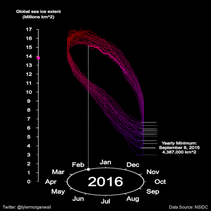
Okay, now let’s generate a title. This functionality is built-in to the rayimage package. Our title will span both images, so it should be 1600 pixels wide.
library(rayimage)
title_mat = matrix(0,70,1600)
title_mat %>%
  add_title(title_text = "Daily Global Sea Ice Total Area with Monthly Polar Sea Ice Extent, 1988-2020",
            title_bar_alpha = 1, title_bar_color = "grey30",
title_color = "white", filename="title") 
Finally: let’s combine all the images together to form our final visualization using magick! We’ll use furrr again to parallelize the process. This function reads the current value for year_val and month_val, and pulls the corresponding render from the world map.
quick_generate_final = function(i) {
  line_image = magick::image_read(glue::glue("seaiceinfo{i}.png"))
  world_image = magick::image_read(glue::glue("seaice_{year_vals[i]}_{month_vals[i]}.png"))

  magick::image_append(c(line_image,world_image)) %>%
    (function(x) magick::image_append(c(title_image,x), stack=TRUE)) %>%
    magick::image_write(glue::glue("full_sea_image{i}.png"))
}
furrr::future_map(1:11924,quick_generate_final)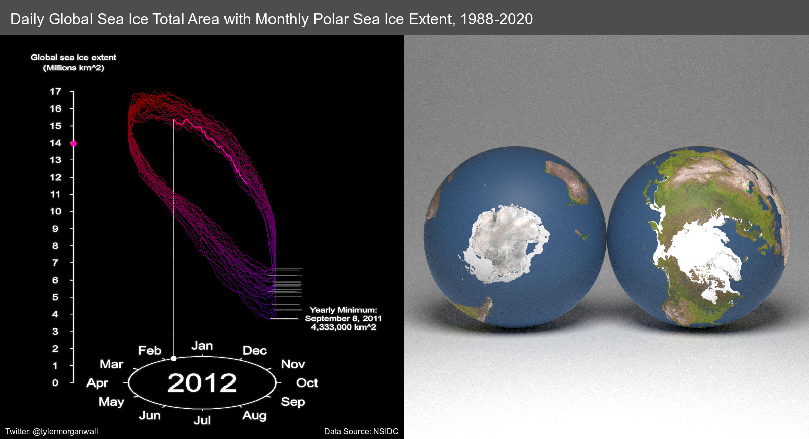
Let’s also repeat the final frame for a few seconds so the reader can take it in.
for(i in 1:180) {
  png::writePNG(png::readPNG("full_sea_image11924.png"),
                glue::glue("full_sea_image{i+11924}.png"))
}
Finally, we’ll use the av package to generate the final video.
av::av_encode_video(glue::glue("full_sea_image{1:12104}.png"),
                    output = "full_sea_viz.mp4", framerate = 60)
I hope you enjoyed this walkthrough! If you want to see more about the thought process I went through when generating the visualization, check out this twitter thread:
2/n I’m going to turn this into a thread where I develop a 3D #dataviz w/ #rayrender/#rstats. A problem with the above viz is it’s unclear it’s 3D—it could be a 2D bean-shaped path. I can rotate around the data, but that introduces new problems: it’s now hard to read the labels. pic.twitter.com/So2WmUMJzk
— Tyler Morgan-Wall (@tylermorganwall) September 26, 2020