A Step-by-Step Guide to Making 3D Maps with Satellite Imagery in R
Ever since I released rayshader to the public, there’s been one question that comes up time and time again: “How do I use rayshader to overlay satellite imagery onto a 3D surface?” And I can see why: 3D maps with real satellite images are super cool, and there are few detailed tutorials out there on how it’s done in R. Additionally, the process behind making this type of map can be intimidating for non-GIS experts, as it exposes you to all complexities of the GIS field: combining different datasets from separate sources—often each with their own distinct coordinate systems—into a single map. Not only that, but you have to also know where and how to get this data—not obvious to someone who doesn’t do this regularly. So I’m going to walk you through how to obtain the data required to make these types of maps, as well as the R code used to generate them. In my opinion, the hardest part is all the manual work in downloading the data! Once that’s done, the code required is short and straightforward, and rayshader makes visualizing elevation data in 3D a breeze. Let’s get started!
First, we’ll download elevation data. A good place to start for reasonable resolution elevation data is the Shuttle Radar Topography Mission (SRTM) dataset. It’s a global 30 meter resolution dataset (meaning, 30m between each point), and although there are more precise and higher resolution datasets out there, few have the global coverage of the SRTM–and it’s dead easy to get the data. Specifically, there’s simple tile selectors out there to download the data by just clicking on a map, which is a far easier process than many other online data repositories.
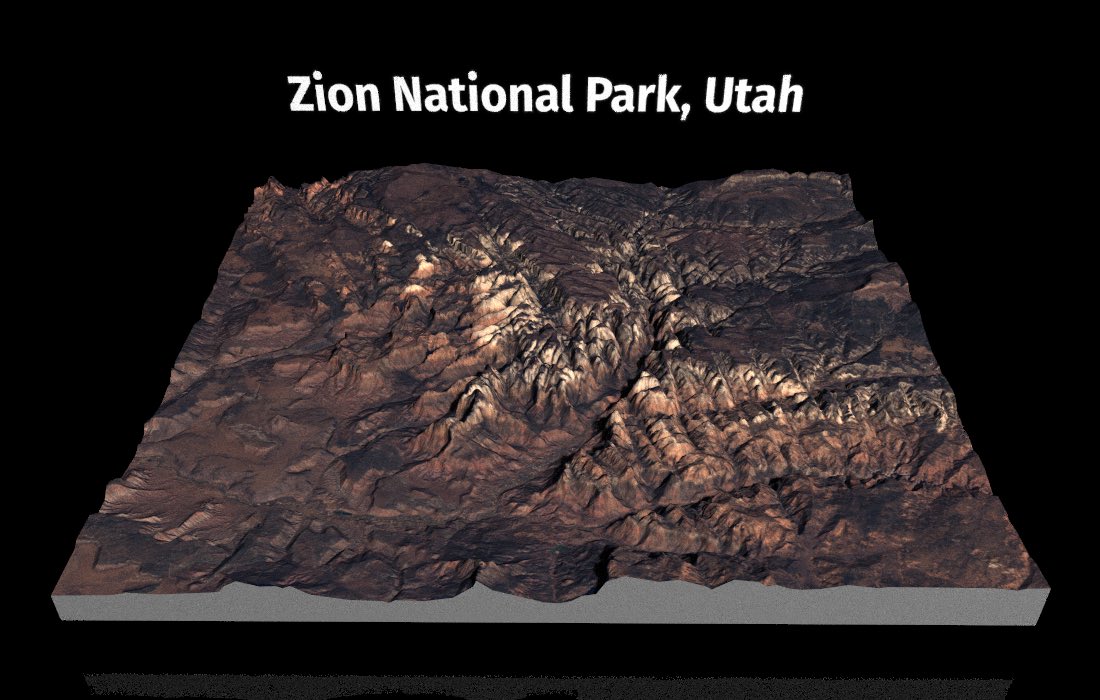
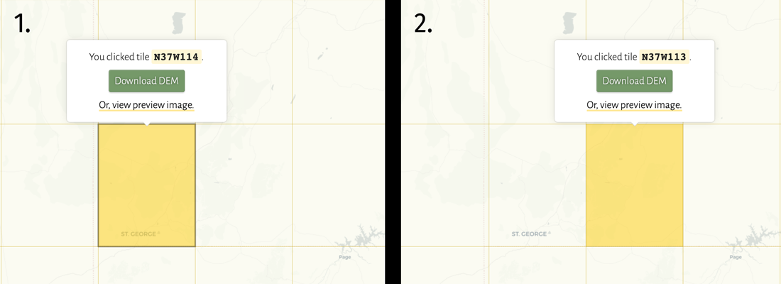
We are going to be visualizing Zion National Park, UT, which has beautiful, dramatic topography. I took a trip with my Dad out to Zion after I finished my PhD, and the gorgeous landscape made up of deep valleys and sheer cliffs makes for an excellent 3D visualization. Let’s start by grabbing elevation data from Derek Watkin’s SRTM tile downloader. We’ll zoom into tiles N37W113.hgt and N37W114.hgt, since the park overlaps both of them. To download: click the tiles, click download, and unzip the files (they should have the file type “hgt”).
Now, we need to get satellite imagery data. This is a bit more involved. There are plenty of sources for this type of data, both paid and freely available. We are going to be taking data from the Landsat 8 project, which does require registering a free USGS account, but then we get access to up-to-date high-quality satellite imagery, for free. So let me walk you through the the step-by-step process to obtain this data.
We are going to go to the USGS Earth Explorer. Once you register an account, you can download datasets. It takes a few minutes to receive your confirmation email, but it comes. Once you get your confirmation email, you can dive right in.
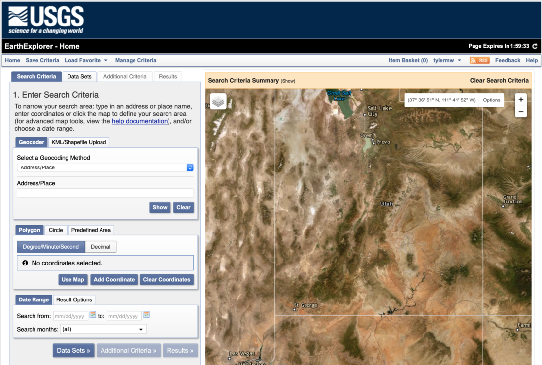
Here’s the interface, with Utah in the viewer. We’re going to zoom in closer to the bottom left corner, which is the location of Zion National Park. Let’s do that:
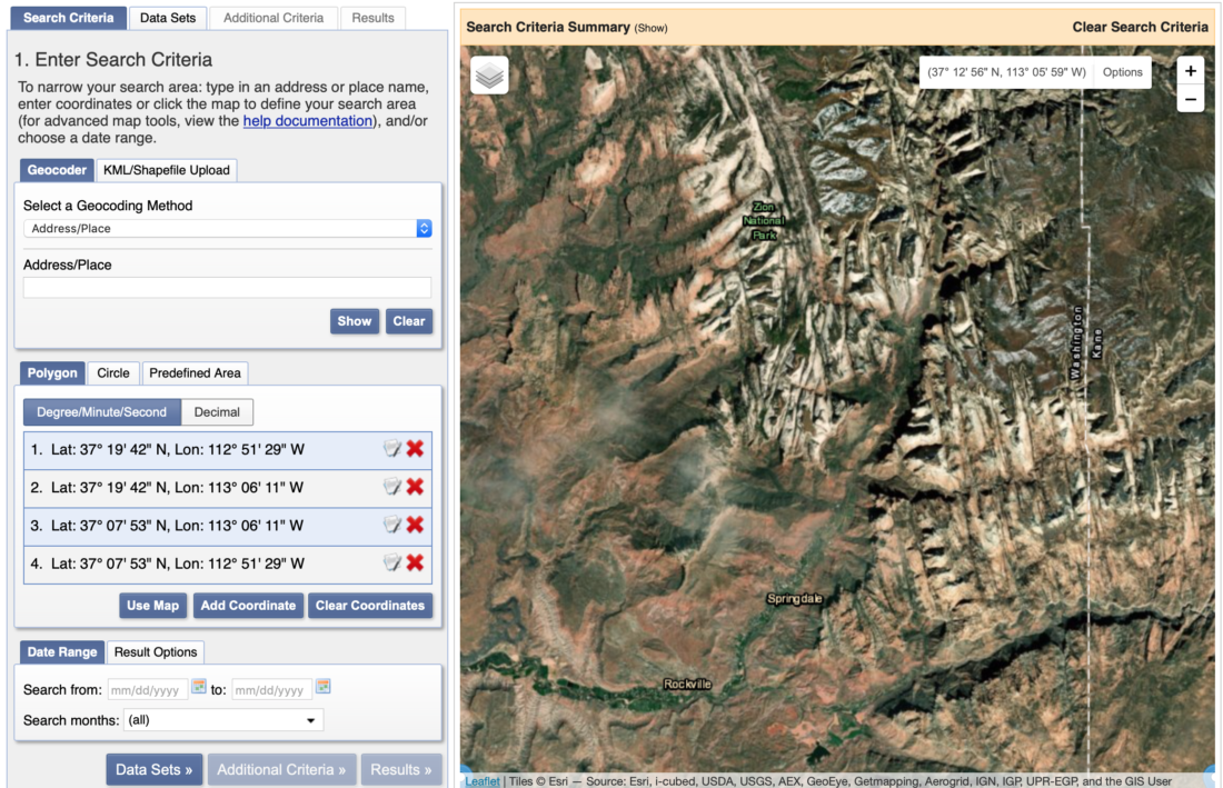
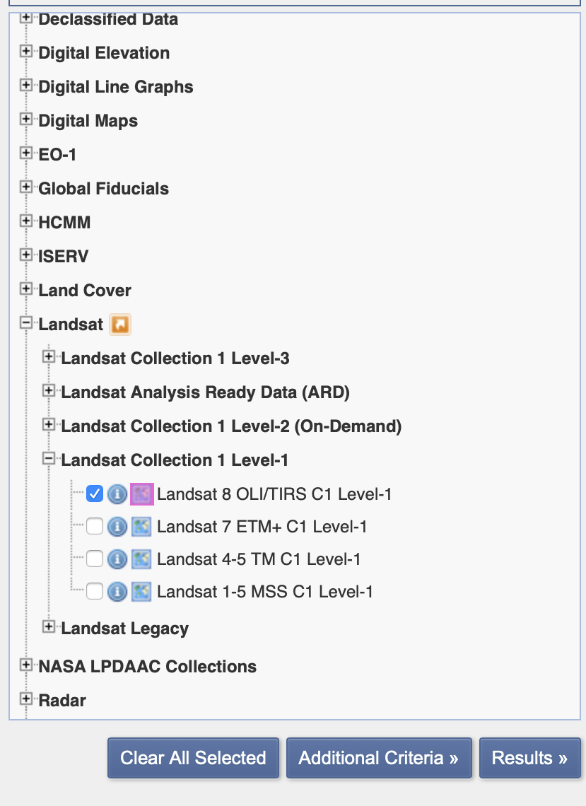
Now that we’re zoomed into the region we want, we’re going to hit the “Use Map” button to mark the current map view as the bounding box for the area we want to search for. We’ll then click “Data Sets” in the bottom left corner. This will query the database and return datasets that include the region we have selected. We specifically want Landsat 8 data, so we’ll select the following:
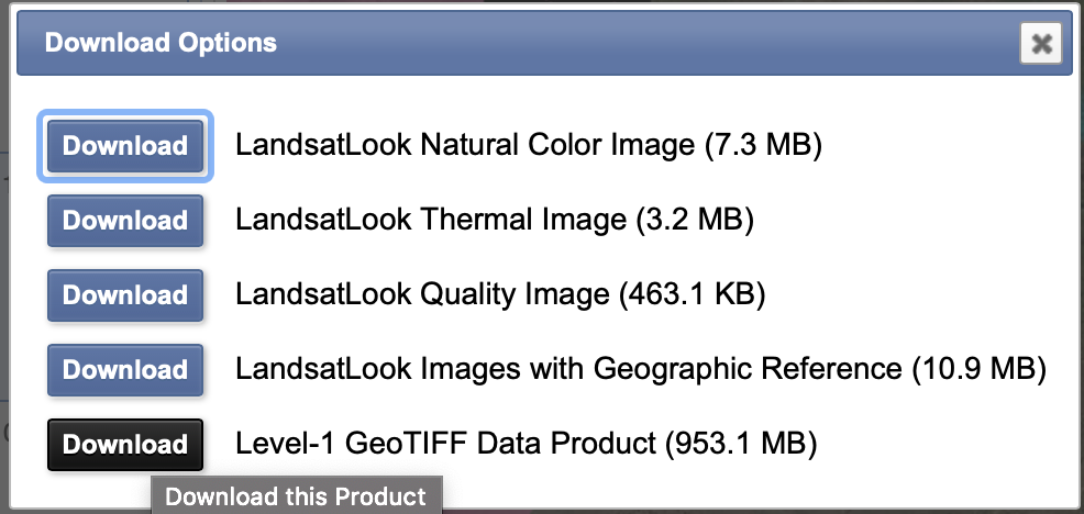
Now, we’ll click “Results”, giving us a list of data products we can select from. If you click the little image icon (second to the left), it will show you a preview of the data in the window to the right. Bluish areas indicate cloud cover, so we’ll flip through the search results until we get a date with a clear shot of the terrain. The first one I find is “LC08_L1TP_038034_20191101_20191114_01_T1”, taken on November 1st, 2019 (or, about 500 years ago in corona-time). Let’s download the full resolution Level 1 GeoTIFF data product (it’s big, almost a gigabyte) and unzip it.
And now–we write our script to turn this into a 3D model! Getting the data was the hardest part. That is, unless you can’t install the following packages–if that’s the case, godspeed, it’s a rite of passage to have to fight with your local GDAL install.
First, let’s load the packages we need. We’ll need rayshader (of course) for 3D plotting, raster for loading and manipulating the data, scale to rescale the color channels to adjust image contrast, and sp to transform some point coordinates between coordinate systems. FYI, I’m using the namespace operator :: throughout the code just to be clear what packages I’m calling from, but you don’t need to do that after you’ve loaded the package with library().
# install.packages(c("rayshader", "raster", "sp"))
library(rayshader)
library(sp)
library(raster)
library(scales)
Let’s load our data. We’ll start with loading the elevation dataset, since it’s an easier process. We’ll use the raster::raster() function to load our SRTM hgt files. This gives us two raster objects. We then combine the two with the raster::merge() function. Since they’re coming from the same data source, we don’t have to worry about transforming coordinate systems to match–they should just merge together seamlessly. We’ll plot the elevation using rayshader::height_shade() so you can see what it looks like:
elevation1 = raster::raster("LC08_L1TP_038034_20191117_20191202_01_T1/N37W113.hgt")
elevation2 = raster::raster("~/Desktop/LC08_L1TP_038034_20191117_20191202_01_T1/N37W114.hgt")

zion_elevation = raster::merge(elevation1,elevation2)

height_shade(raster_to_matrix(zion_elevation)) %>%
  plot_map()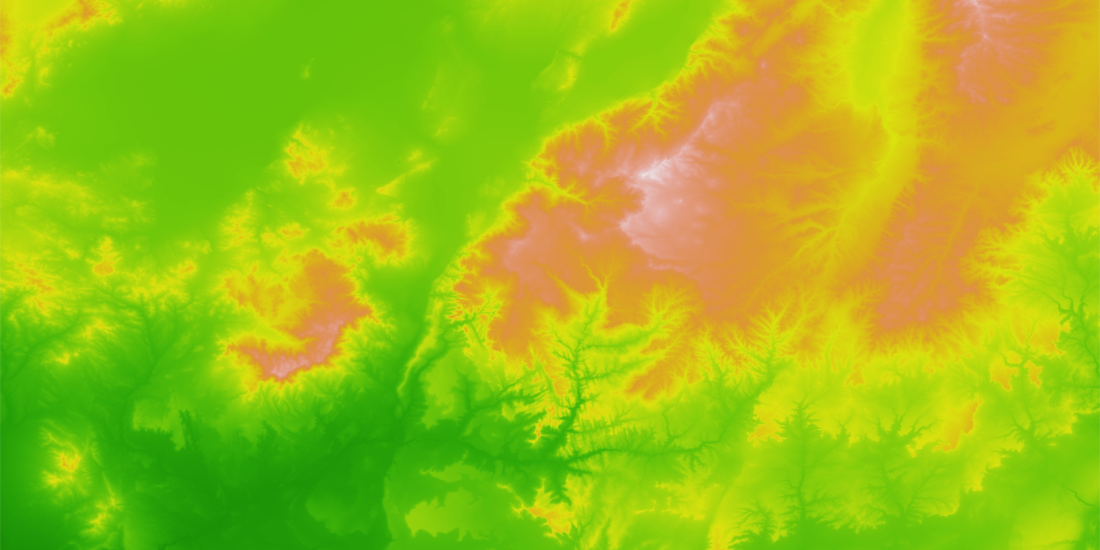
height_shade() function. Zion National Park is in the center.
Great! Now, let’s load our georeferenced satellite imagery. The red, blue, and green bands on Landsat 8 data are bands B4, B3, and B2, respectively. You can delete the rest of the bands if you want to free 600 megabytes of space on your hard drive. Let’s then plot it with raster::plotRGB().
zion_r = raster::raster("LC08_L1TP_038034_20191117_20191202_01_T1_B4.TIF")
zion_g = raster::raster("LC08_L1TP_038034_20191117_20191202_01_T1_B3.TIF")
zion_b = raster::raster("LC08_L1TP_038034_20191117_20191202_01_T1_B2.TIF")

zion_rbg = raster::stack(zion_r, zion_g, zion_b)
raster::plotRGB(zion_rbg, scale=255^2)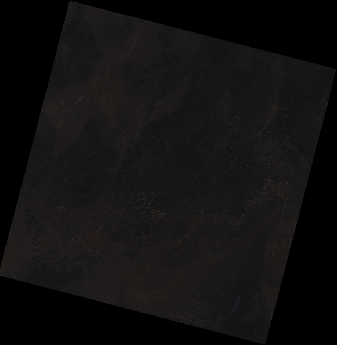
Why is it so dark? We need to apply a gamma correction to the the imagery, which corrects raw linear intensity data for our non-linear perception of darkness. We do that simply by taking the square root of the data (we can also remove the scale argument).
zion_rbg_corrected = sqrt(raster::stack(zion_r, zion_g, zion_b))
raster::plotRGB(zion_rbg_corrected)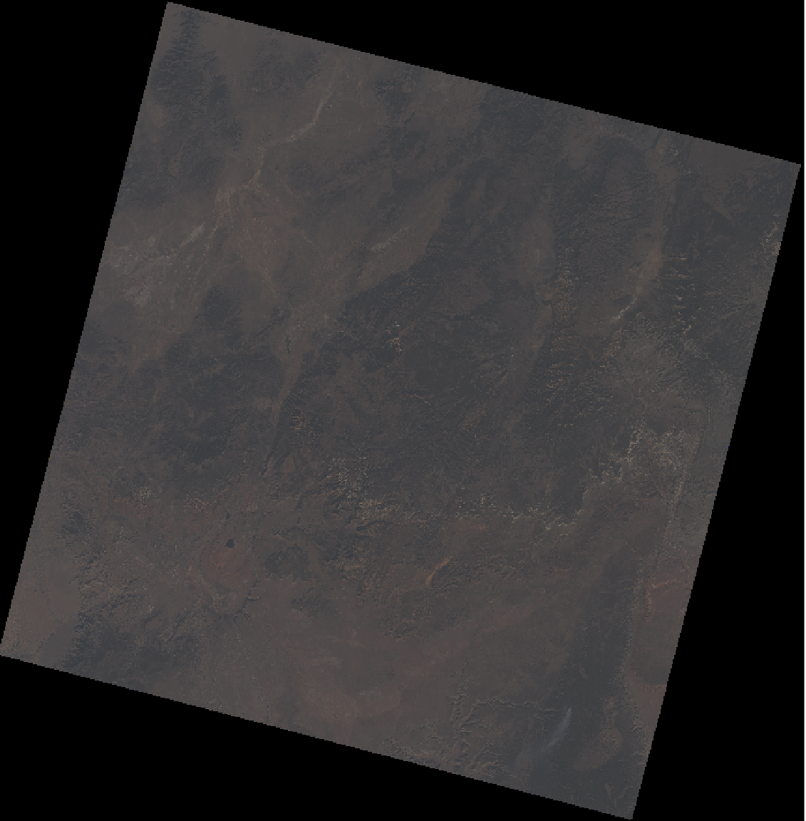
Great! The contrast is muted, but we’ll fix that later. Now, let’s combine the two datasets. Here we encounter our first GIS difficulty: the coordinate reference systems of our elevation data and imagery data don’t match! Oh no.
raster::crs(zion_r)## CRS arguments:
## +proj=utm +zone=12 +datum=WGS84 +units=m +no_defs +ellps=WGS84
## +towgs84=0,0,0raster::crs(zion_elevation)## CRS arguments:
## +proj=longlat +datum=WGS84 +no_defs +ellps=WGS84 +towgs84=0,0,0
Our imagery data is given in UTM coordinates, while our elevation is in long/lat. Thankfully, it’s fairly straightforward to transform the elevation data from long/lat to UTM with the raster::projectRaster() function. We use the “bilinear” method for interpolation since elevation is a continuous variable.
crs(zion_r)## CRS arguments:
## +proj=utm +zone=12 +datum=WGS84 +units=m +no_defs +ellps=WGS84
## +towgs84=0,0,0zion_elevation_utm = raster::projectRaster(zion_elevation, crs = crs(zion_r), method = "bilinear")
crs(zion_elevation_utm)## CRS arguments:
## +proj=utm +zone=12 +datum=WGS84 +units=m +no_defs +ellps=WGS84
## +towgs84=0,0,0
Now, let’s crop the region down to the park itself. To figure out what long/lat values enclosed our area, I went to Google Maps and double clicked on the map to extract the bottom left and top right corners of the bounding box for the final map. We’ll use the sp package to transform these long/lat coords into UTM coordinates.
bottom_left = c(y=-113.155277, x=37.116253)
top_right   = c(y=-112.832502, x=37.414948)

extent_latlong = sp::SpatialPoints(rbind(bottom_left, top_right), proj4string=sp::CRS("+proj=longlat +ellps=WGS84 +datum=WGS84"))
extent_utm = sp::spTransform(extent_latlong, raster::crs(zion_elevation_utm))

e = raster::extent(extent_utm)
e
## class : Extent
## xmin : 308511.9
## xmax : 337834.2
## ymin : 4109943
## ymax : 4142481
Now we’ll crop our datasets to the same region, and create an 3-layer RGB array of the image intensities. This is what rayshader needs as input to drape over the elevation values. We also need to transpose the array, since rasters and arrays are oriented differently in R, because of course they are🙄. We do that with the aperm() function, which performs a multi-dimensional transpose. We’ll also convert our elevation data to a base R matrix, which is what rayshader expects for elevation data.
zion_rgb_cropped = raster::crop(zion_rbg_corrected, e)
elevation_cropped = raster::crop(zion_elevation_utm, e)

names(zion_rgb_cropped) = c("r","g","b")

zion_r_cropped = rayshader::raster_to_matrix(zion_rgb_cropped$r)
zion_g_cropped = rayshader::raster_to_matrix(zion_rgb_cropped$g)
zion_b_cropped = rayshader::raster_to_matrix(zion_rgb_cropped$b)

zionel_matrix = rayshader::raster_to_matrix(elevation_cropped)

zion_rgb_array = array(0,dim=c(nrow(zion_r_cropped),ncol(zion_r_cropped),3))

zion_rgb_array[,,1] = zion_r_cropped/255 #Red layer
zion_rgb_array[,,2] = zion_g_cropped/255 #Blue layer
zion_rgb_array[,,3] = zion_b_cropped/255 #Green layer

zion_rgb_array = aperm(zion_rgb_array, c(2,1,3))

plot_map(zion_rgb_array)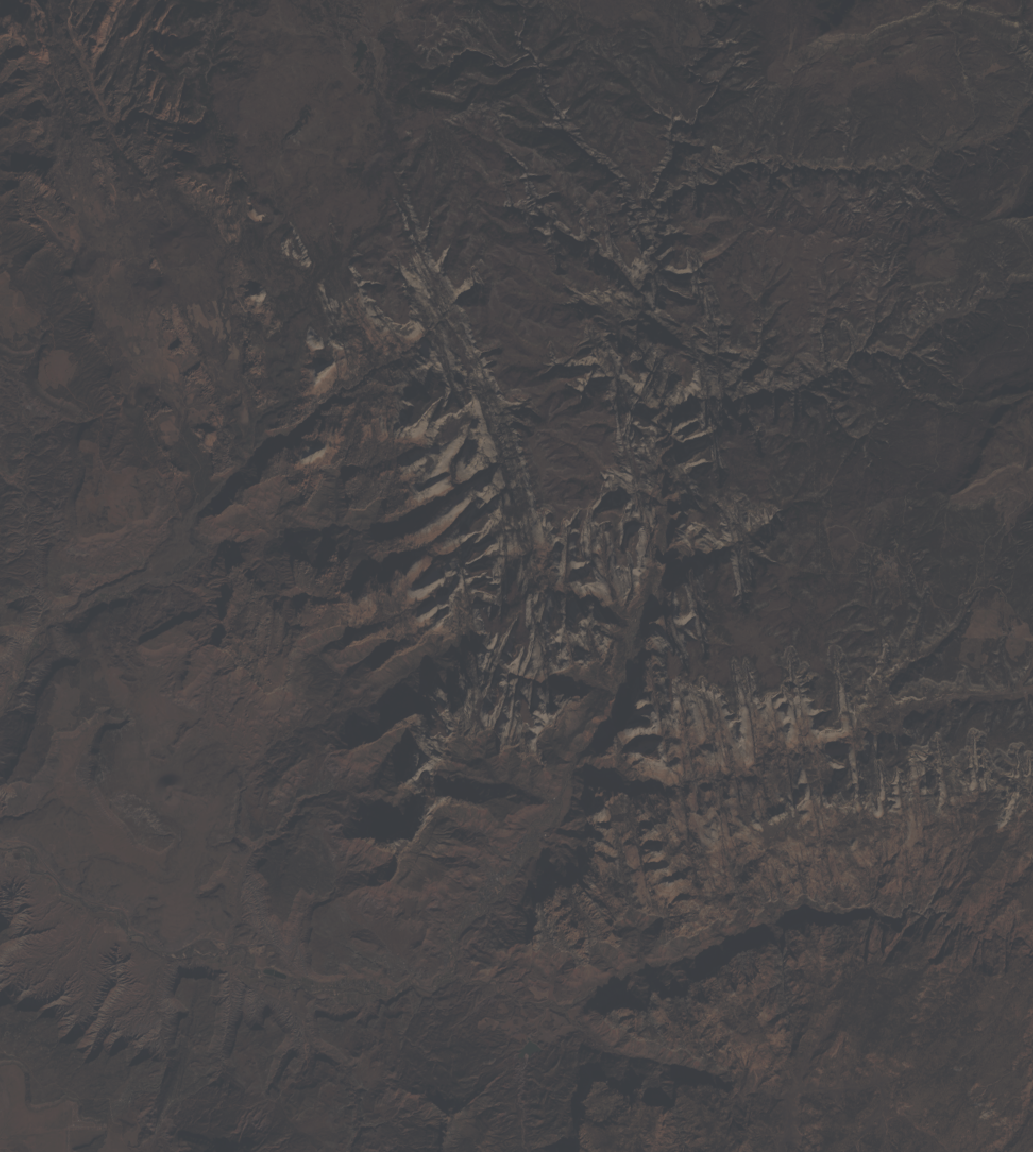
We will also now scale our data to improve the contrast and make the image more vibrant. I’m going to use the scales package to rescale the image to use the full range of color.
zion_rgb_contrast = scales::rescale(zion_rgb_array,to=c(0,1))

plot_map(zion_rgb_contrast)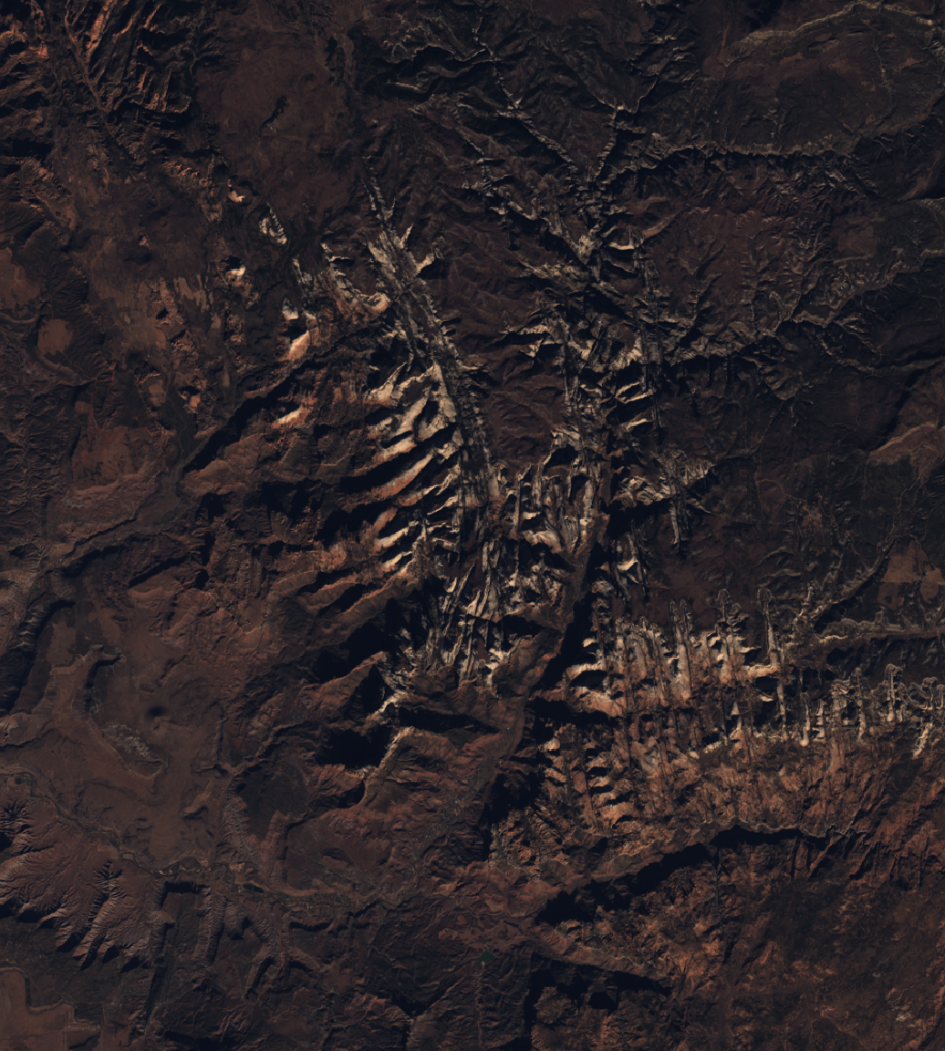
Excellent. Now we just input this image into plot_3d() along with our elevation data. For a realistic landscape, we should set zscale = 30 (since the elevation data was taken at 30 meter increments), but we’re going to set zscale = 15 to give the landscape 2x exaggeration. If you’re following along, you should now have an rgl window open with a 3D model you can rotate around.
plot_3d(zion_rgb_contrast, zionel_matrix, windowsize = c(1100,900), zscale = 15, shadowdepth = -50,
        zoom=0.5, phi=45,theta=-45,fov=70, background = "#F2E1D0", shadowcolor = "#523E2B")
render_snapshot(title_text = "Zion National Park, Utah | Imagery: Landsat 8 | DEM: 30m SRTM",
                title_bar_color = "#1f5214", title_color = "white", title_bar_alpha = 1)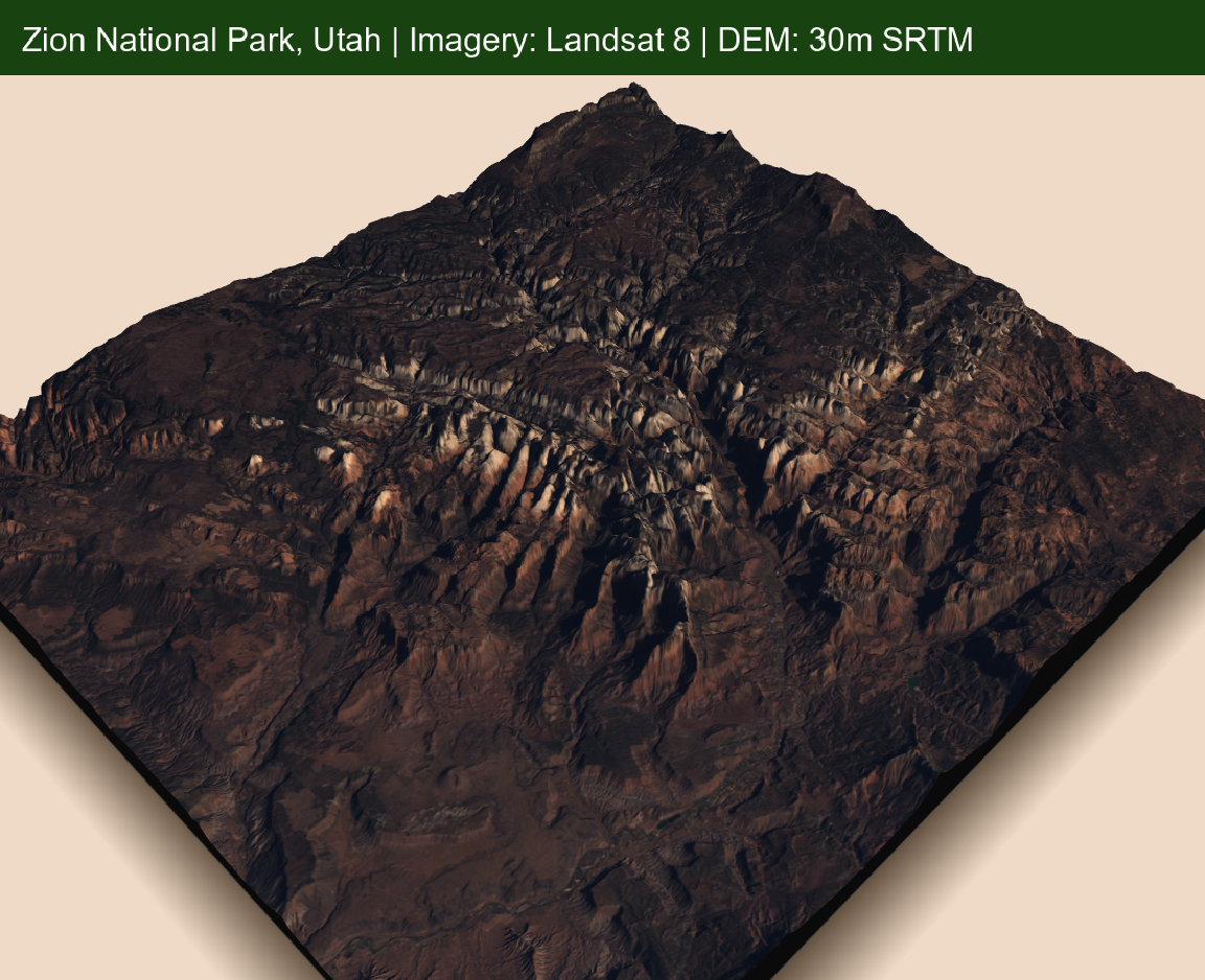
The static snapshot above is nice, but 3D is best seen in motion, so let’s create a movie of us rotating around the scene. We’ll move the camera with render_camera(), and generate 1440 frames with render_snapshot(). At 60 frames per second, this will generate a 24 second video. You can do this via the av package, but I’m going to call ffmpeg directly via a system() call, since the output of av doesn’t seem to play nicely with embeddable web videos (for some reason).
angles= seq(0,360,length.out = 1441)[-1]
for(i in 1:1440) {
  render_camera(theta=-45+angles[i])
  render_snapshot(filename = sprintf("zionpark%i.png", i),
                  title_text = "Zion National Park, Utah | Imagery: Landsat 8 | DEM: 30m SRTM",
                  title_bar_color = "#1f5214", title_color = "white", title_bar_alpha = 1)
}
rgl::rgl.close()

#av::av_encode_video(sprintf("zionpark%d.png",seq(1,1440,by=1)), framerate = 30,
                    # output = "zionpark.mp4")

rgl::rgl.close()
system("ffmpeg -framerate 60 -i zionpark%d.png -pix_fmt yuv420p zionpark.mp4")
And we’re done! What to do now? Well, this satellite imagery and elevation data is relatively low resolution–you could now search for higher resolution imagery and elevation data to produce a more detailed figure. The general process is the same for any data source: find the data, transform the data into a common coordinate system, crop the data to the desired region, and then combine the data in plot_3d(). You could also try using the ender_highquality() function in rayshader to make beautiful, pathtraced maps (like in the featured animation at the top of the page). Or you could learn more about using rayshader (include transforming LIDAR point data to extremely hi-res elevation data) in my masterclass: the materials are free and open source. And this blog post is by no means the authoritative source on how to do this: there are lots of packages and free books on remote sensing and GIS. Have fun!
And whatever you end up doing, if you create something cool be sure to tweet it with the hashtags #rstats and #rayshader! We’d all love to see what you’ve created.