Tutorial: Adding Open Street Map Data to Rayshader Maps in R
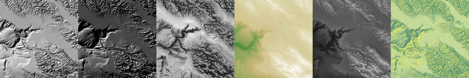
This post is a tutorial on how to add Open Street Map data to maps made with rayshader in R. Rayshader is a package for 2D and 3D visualization in R, specializing in generating beautiful maps using many various hillshading techniques (see these posts [1] [2] [3]) directly from elevation data. It does this by providing the user with a wide variety of techniques: traditional lambertian shading, raytracing, ambient occlusion, hypsometric tinting (cartography-speak for mapping color to elevation), texture shading, and spherical aspect color shading.
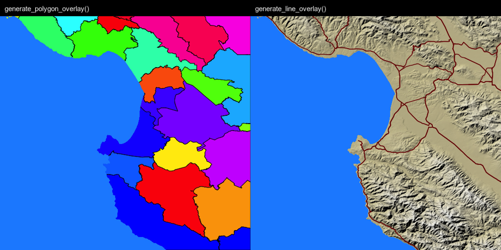
These techniques can be combined to create stunning maps in a few lines of R code, but that’s only half the story: a beautiful map is just a vehicle to deliver other information. Roads, trails, parking lots, water fountains, restrooms, the nearest Arbys: a map is a tool to build your mental model for a region. These features can be added to rayshader maps via data overlays: we first generate our base map using some combination of the above hillshading techniques, and then we layer our data on top. Rayshader provides you with functions to easily add polygons, lines, and points that represent your data directly onto your map.
You also need a source of data, and luckily we live in a universe where Open Street Map (OSM) exists: a free, open, user-generated map of pretty much everything in the world. If you have some highly specialized dataset, you might not be able to find it on OSM, but for the basics (trails, roads, rivers, streams, landmarks and buildings) it’s fairly comprehensive.
Knowing the data exists is only half the battle: you also need a way to load the data into R. And thankfully, Mark Padgham (along with many others and the rOpenSci project) have given us the osmdata package, a package that allows you to easily query and pull data from OSM in a few lines of code directly from R. You provide it with a lat/long bounding box and a specific feature you want to pull, and it will return an object containing everything that matches your query in that area.
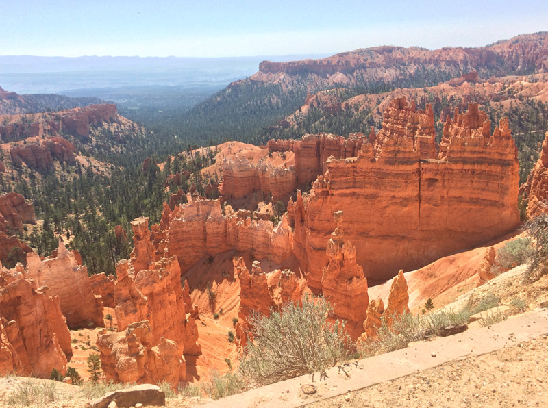
Let’s jump into an example. We’ll use elevation data from Bryce Canyon in Utah (courtesy of Tom Patterson via shadedrelief.com), since National Parks tend to have a nice mix of interesting topography, trails, streams, and other features.
Let’s start by loading the data and required packages. We’ll transform the spatial data structure extracted by raster into a regular R matrix using rayshader’s raster_to_matrix() function.
install.packages("remotes")
remotes::install_github("tylermorganwall/rayshader")
remotes::install_github("tylermorganwall/rayimage")

library(rayshader)
library(raster)
library(osmdata)
library(sf)
library(dplyr)
library(ggplot2)

bryce = raster("Bryce_Canyon.tif")
bryce_mat = raster_to_matrix(bryce)
We can also create a smaller version of this matrix for quick prototyping with the rayshader resize_matrix() function. This test matrix will be 1/4th the size of the full matrix.
bryce_small = resize_matrix(bryce_mat,0.25)Now, let’s build our base map with rayshader. Let’s see what this data looks like with a basic color to elevation mapping.
bryce_small %>%
  height_shade() %>%
  plot_map()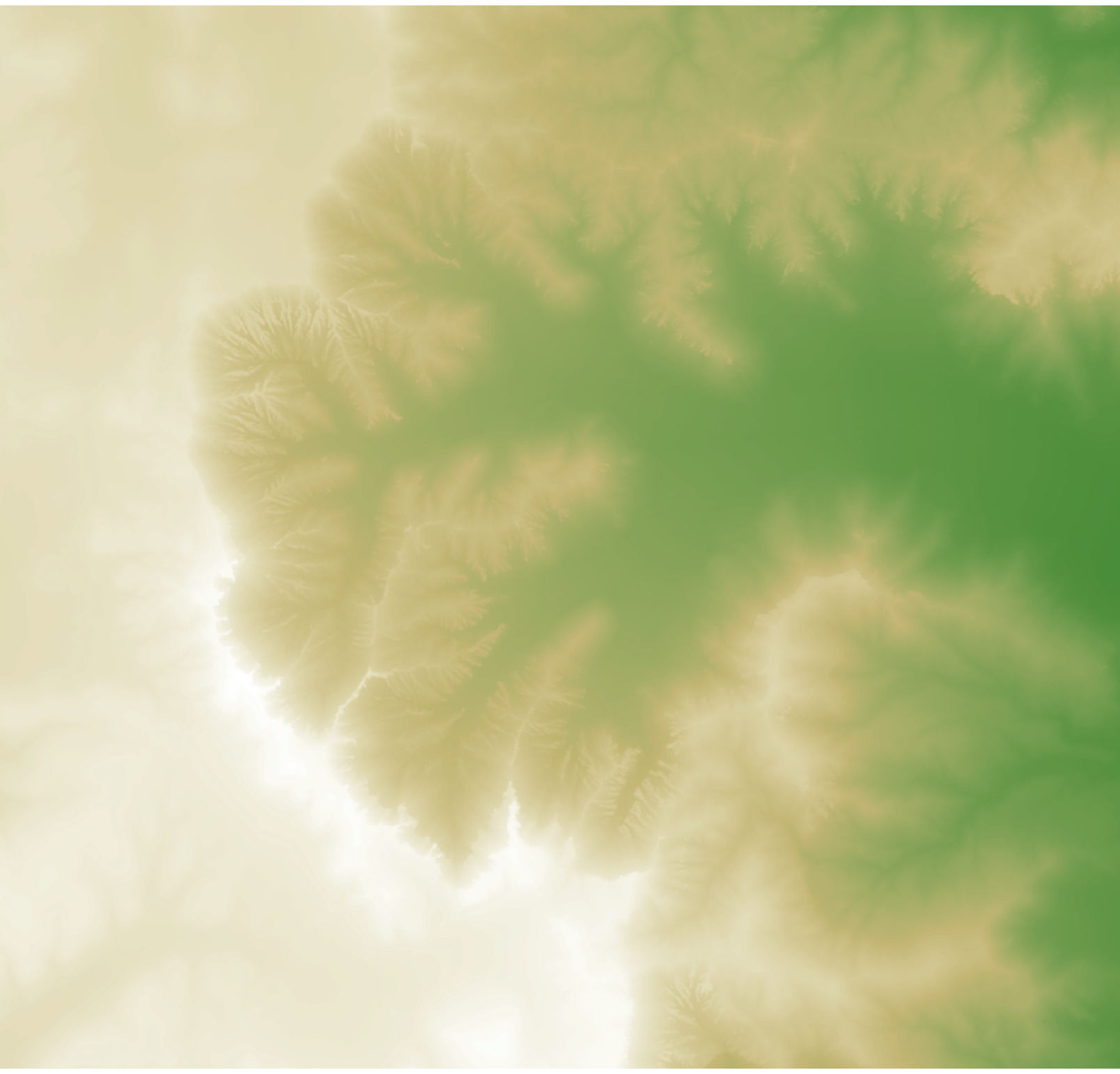
We’ll mix this layer with a spherical aspect shading color layer to enhance it using sphere_shade().
bryce_small %>%
  height_shade() %>%
  add_overlay(sphere_shade(bryce_small, texture = "desert",
                           zscale=4, colorintensity = 5), alphalayer=0.5) %>%
  plot_map()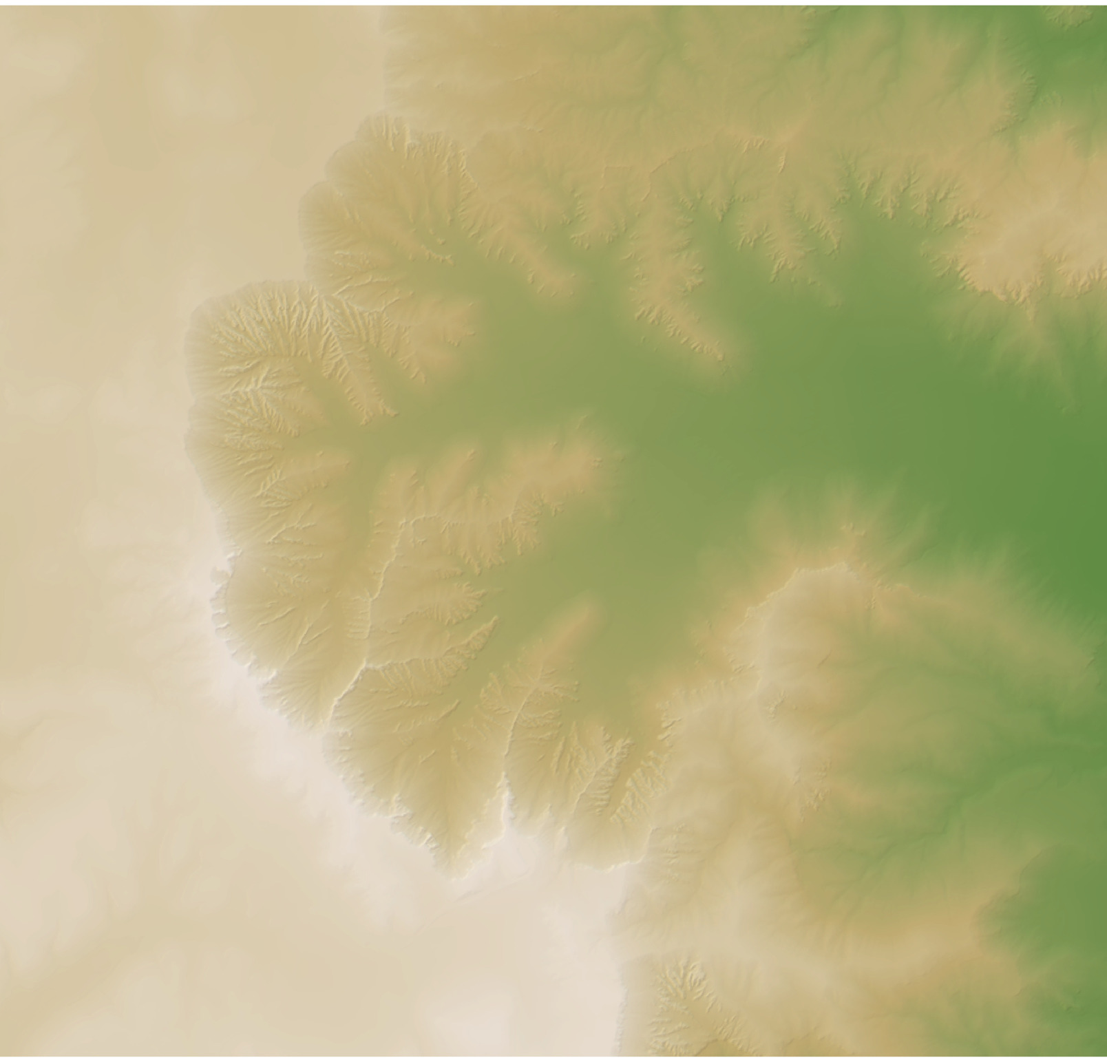
We can also overlay a standard hillshade to better define the terrain. We’ll get this by using the lamb_shade() function, which adds Lambertian (cosine) shading. The zscale parameter in lamb_shade() controls the amount of vertical exaggeration and thus the intensity of the hillshade.
bryce_small %>%
  height_shade() %>%
  add_overlay(sphere_shade(bryce_small, texture = "desert",
                           zscale=4, colorintensity = 5), alphalayer=0.5) %>%
  add_shadow(lamb_shade(bryce_small,zscale = 6),0) %>%
  plot_map()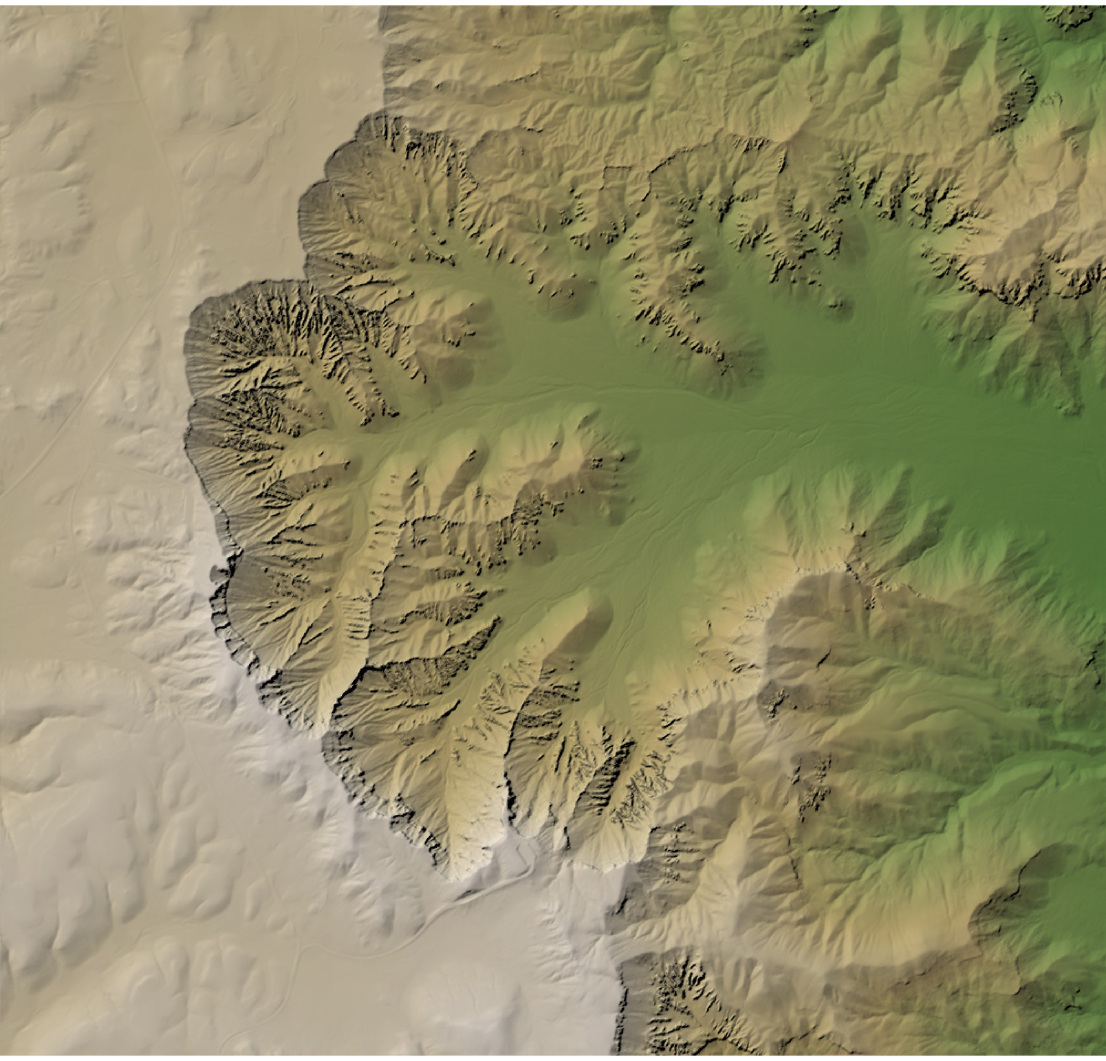
Now we’ll add a layer using the texture_shade() function, which adds shadows calculated by Leland Brown’s “texture shading” method. This better defines ridges and drainage networks, which aren’t well-captured by Lambertian shading.
bryce_small %>%
  height_shade() %>%
  add_overlay(sphere_shade(bryce_small, texture = "desert",
                           zscale=4, colorintensity = 5), alphalayer=0.5) %>%
  add_shadow(lamb_shade(bryce_small,zscale=6), 0) %>%
  add_shadow(texture_shade(bryce_small,detail=8/10,contrast=9,brightness = 11), 0.1) %>%
  plot_map()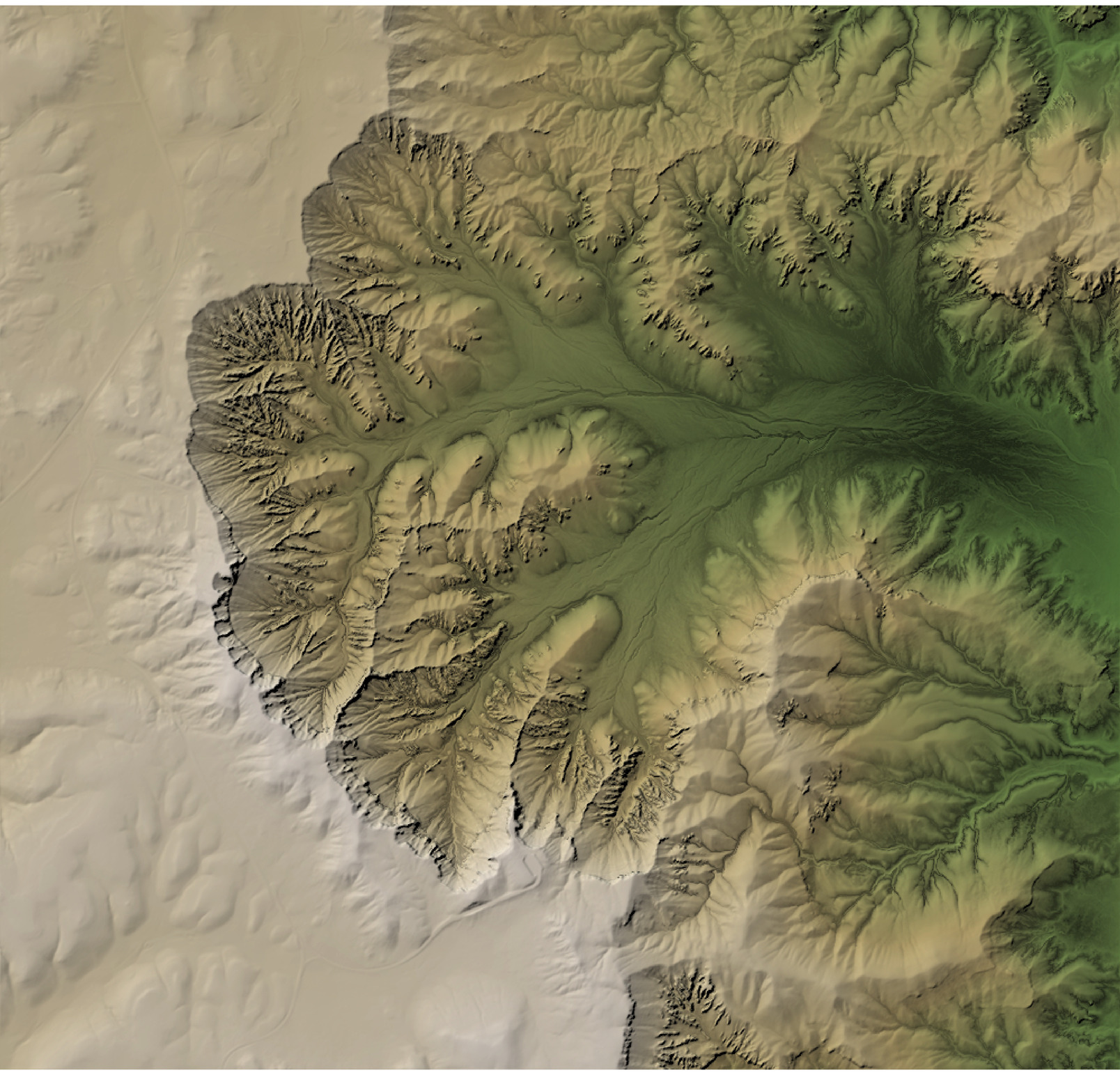
Finally, we’ll add an ambient occlusion layer to our base map. This will darken valleys to account for less scattered atmospheric light reaching the valley floor. This adds a nice texture to our map, particularly to the valleys between the steep ridges.
bryce_small %>%
  height_shade() %>%
  add_overlay(sphere_shade(bryce_small, texture = "desert",
                           zscale=4, colorintensity = 5), alphalayer=0.5) %>%
  add_shadow(lamb_shade(bryce_small,zscale=6), 0) %>%
  add_shadow(ambient_shade(bryce_small), 0) %>%
  add_shadow(texture_shade(bryce_small,detail=8/10,contrast=9,brightness = 11), 0.1) %>%
  plot_map()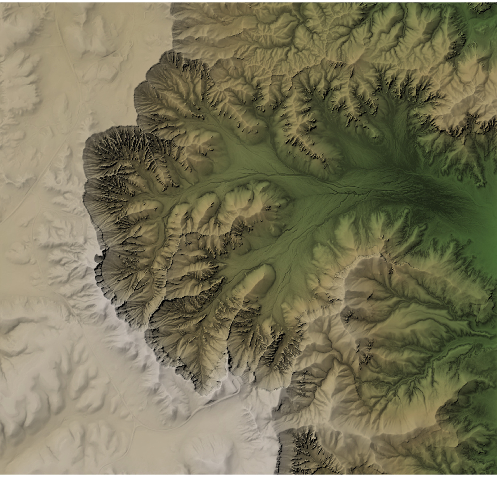
Now we have our base map! We’ll zoom into our area of interest by creating a lat/long bounding box. To get these coordinates, I just went to Google Maps and picked the bottom left and top right corners, and pulled out the lat/long values. I wrote a short function that takes these values and transforms them into the coordinate system used in the original bryce object, which we then crop, convert to a matrix, and then plot. We’ll also save this map to a variable to use later, so we don’t have to recompute the base layer each time.
lat_range   = c(37.614998, 37.629084)
long_range = c(-112.174228, -112.156230)

convert_coords = function(lat,long, from = CRS("+init=epsg:4326"), to) {
  data = data.frame(long=long, lat=lat)
  coordinates(data) <- ~ long+lat
  proj4string(data) = from
  #Convert to coordinate system specified by EPSG code
  xy = data.frame(sp::spTransform(data, to))
  colnames(xy) = c("x","y")
  return(unlist(xy))
}

crs(bryce)
## CRS arguments:
## +proj=utm +zone=12 +ellps=GRS80 +towgs84=0,0,0,0,0,0,0 +units=m
## +no_defutm_bbox = convert_coords(lat = lat_range, long=long_range, to = crs(bryce))
utm_bbox## x1 x2 y1 y2
## 396367.4 397975.2 4163747.9 4165291.0extent(bryce)## class : Extent
## xmin : 395998.5
## xmax : 399998.5
## ymin : 4161774
## ymax : 4165574extent_zoomed = extent(utm_bbox[1], utm_bbox[2], utm_bbox[3], utm_bbox[4])
bryce_zoom = crop(bryce, extent_zoomed)
bryce_zoom_mat = raster_to_matrix(bryce_zoom)
base_map = bryce_zoom_mat %>%
height_shade() %>%
add_overlay(sphere_shade(bryce_zoom_mat, texture = "desert", colorintensity = 5), alphalayer=0.5) %>%
add_shadow(lamb_shade(bryce_zoom_mat), 0) %>%
add_shadow(ambient_shade(bryce_zoom_mat),0) %>%
add_shadow(texture_shade(bryce_zoom_mat,detail=8/10,contrast=9,brightness = 11), 0.1)
plot_map(base_map)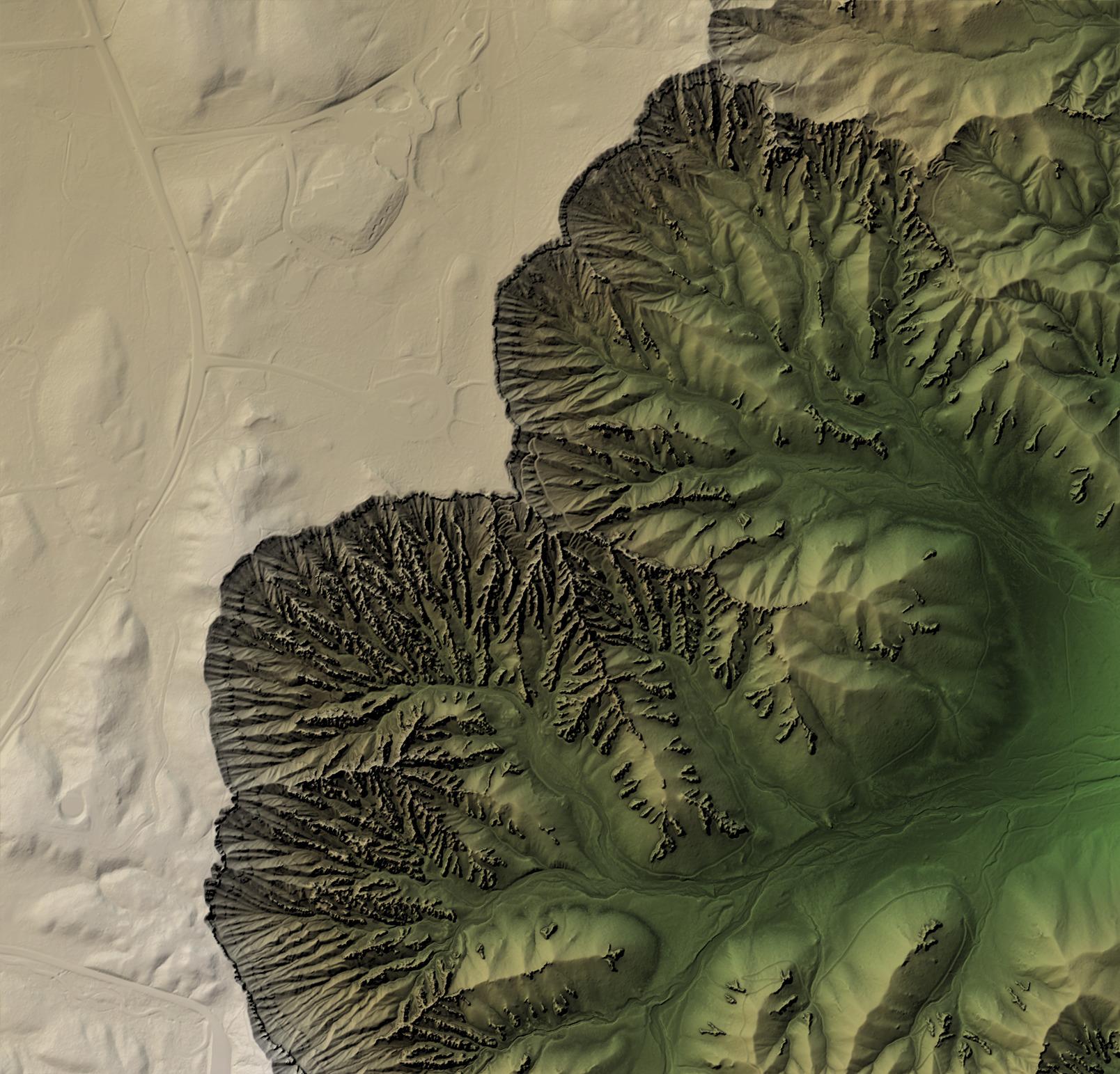
Great! We now have our zoomed-in base map. Let’s start adding OSM features to it.
You can see what features are available in OSM by calling the available_features() function. We’re first going to pull the highway feature in our region. Despite the name, highway represents more than major roads: it’s a feature that represents all types of roads and footpaths. We’ll build a query to the OSM Overpass API by passing in our lat/long bounding box (with a slight order change required for that API) to opq(), adding a feature with add_osm_feature(), and then convert the object to a simple features (sf) object with osmdata_sf().
osm_bbox = c(long_range[1],lat_range[1], long_range[2],lat_range[2])

bryce_highway = opq(osm_bbox) %>%
  add_osm_feature("highway") %>%
  osmdata_sf()
bryce_highway
## Object of class 'osmdata' with:
## $bbox : 37.614998,-112.174228,37.629084,-112.15623
## $overpass_call : The call submitted to the overpass API
## $meta : metadata including timestamp and version numbers
## $osm_points : 'sf' Simple Features Collection with 2140 points
## $osm_lines : 'sf' Simple Features Collection with 94 linestrings
## $osm_polygons : 'sf' Simple Features Collection with 5 polygons
## $osm_multilines : NULL
## $osm_multipolygons : NULL
This returns a list with several sf objects contained within: points, lines, and polygons. The data comes in lat/long coordinates, so we need to convert it to bryce’s coordinate system. Let’s plot the lines in ggplot to preview what data we have.
bryce_lines = st_transform(bryce_highway$osm_lines, crs=crs(bryce))

ggplot(bryce_lines,aes(color=osm_id)) +
  geom_sf() +
  theme(legend.position = "none") +
  labs(title = "Open Street Map `highway` attribute in Bryce Canyon National Park")
Now, let’s add it to our map using rayshader’s generate_line_overlay() function, which takes an sf object with LINESTRING geometry and creates a semi-transparent overlay (which we then overlay with add_overlay()). You might notice that the above geometry extends far beyond the bounds of our scene, but that won’t matter—the generate_*_overlay() functions will crop the data down the region specified in extent.
base_map %>%
  add_overlay(generate_line_overlay(bryce_lines,extent = extent_zoomed,
                                    heightmap = bryce_zoom_mat)) %>%
  plot_map()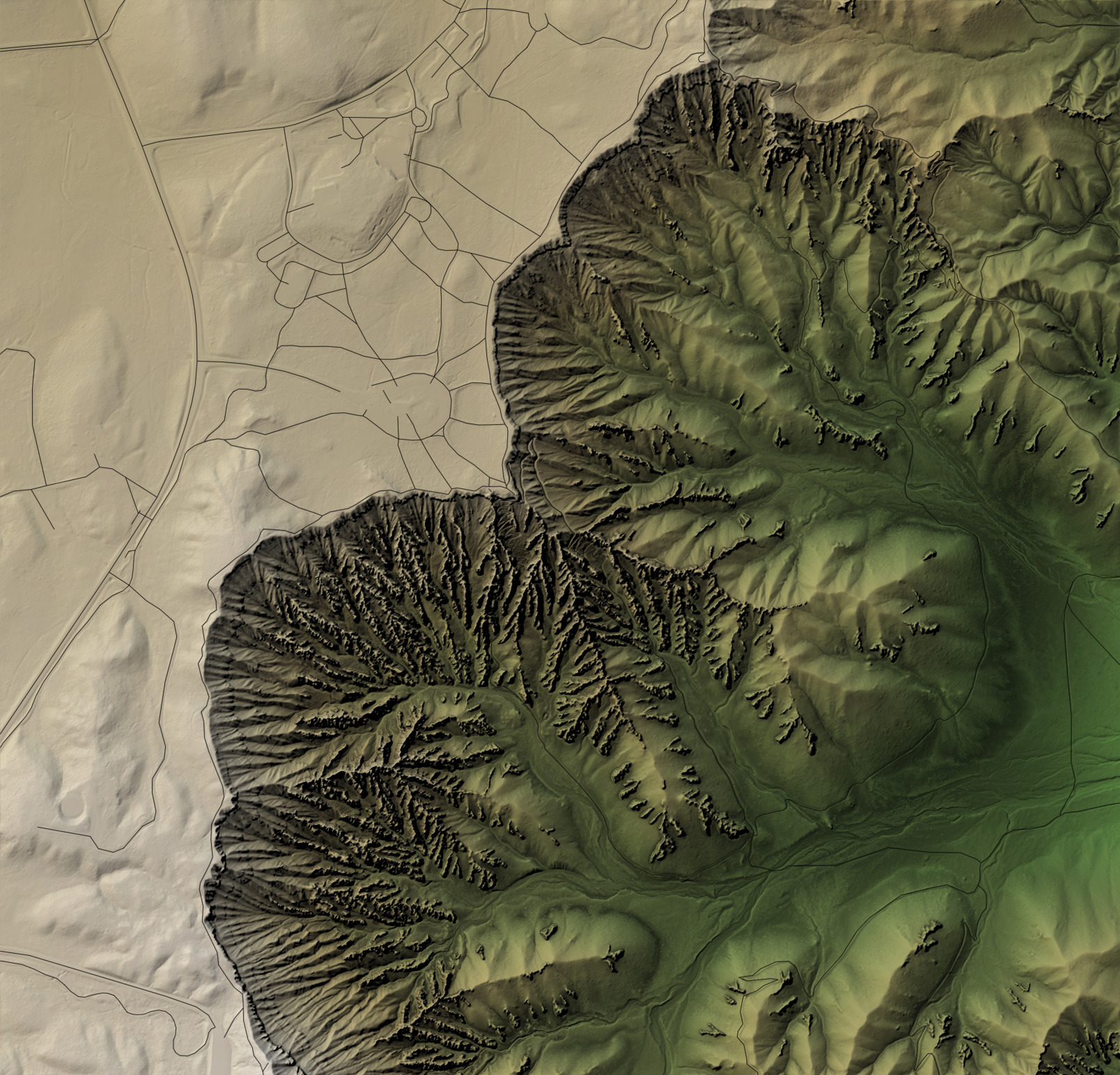
Great! We have road and trails. Let’s make the lines white and a bit thicker.
base_map %>%
  add_overlay(generate_line_overlay(bryce_lines,extent = extent_zoomed,
                                    linewidth = 3, color="white",
                                    heightmap = bryce_zoom_mat)) %>%
  plot_map()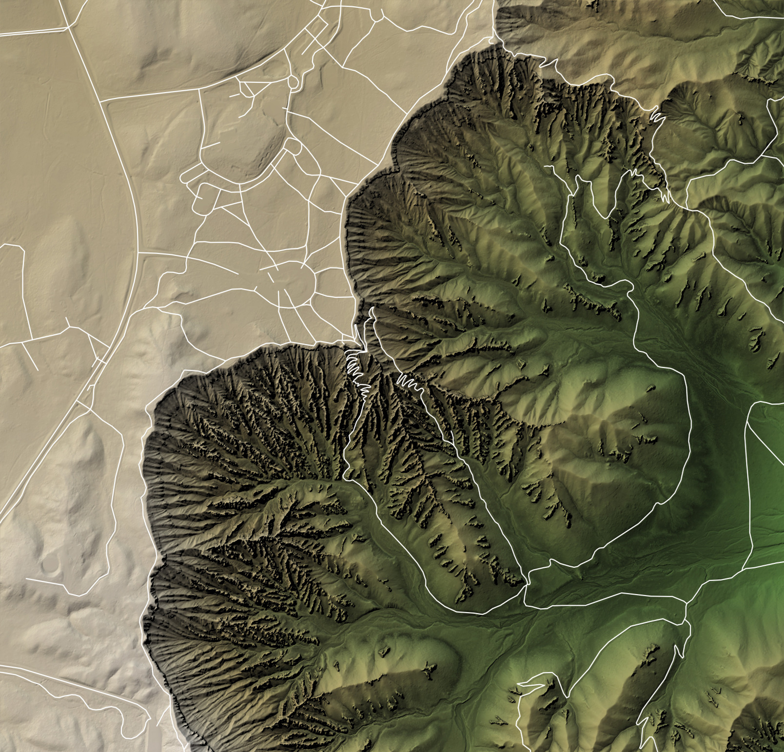
Now, let’s filter them into several different categories. We’ll first separate out roads, footpaths, and trails using dplyr’s filter() function.
bryce_trails = bryce_lines %>%
  filter(highway %in% c("path","bridleway"))

bryce_footpaths = bryce_lines %>%
  filter(highway %in% c("footway"))

bryce_roads = bryce_lines %>%
  filter(highway %in% c("unclassified", "secondary", "tertiary", "residential", "service"))
Let’s plot them all together. We’ll vary the color, line width, and line type (argument lty) to differentiate the different paths. We’ll use thick dark lines for roads, solid white lines for paved paths, and dotted white lines for trails.
base_map %>%
  add_overlay(generate_line_overlay(bryce_footpaths,extent = extent_zoomed,
                                    linewidth = 6, color="white",
                                    heightmap = bryce_zoom_mat)) %>%
  add_overlay(generate_line_overlay(bryce_trails,extent = extent_zoomed,
                                    linewidth = 3, color="white", lty=3,
                                    heightmap = bryce_zoom_mat)) %>%
  add_overlay(generate_line_overlay(bryce_roads,extent = extent_zoomed,
                                    linewidth = 8, color="black",
                                    heightmap = bryce_zoom_mat)) %>%
  plot_map()
One problem with light colored lines on light backgrounds is lack of contrast: it can be harder to see the white lines in areas where the base map is also light. This particular issue can be fixed by adding a slight outline to our light lines. We can create an outline by plotting the same data twice, changing the color and decreasing the line width for the second layer.
We’ll try this with the foot paths.
base_map %>%
  add_overlay(generate_line_overlay(bryce_footpaths,extent = extent_zoomed,
                                    linewidth = 10, color="black",
                                    heightmap = bryce_zoom_mat)) %>%
  add_overlay(generate_line_overlay(bryce_footpaths,extent = extent_zoomed,
                                    linewidth = 6, color="white",
                                    heightmap = bryce_zoom_mat)) %>%
  add_overlay(generate_line_overlay(bryce_trails,extent = extent_zoomed,
                                    linewidth = 3, color="white", lty=3,
                                    heightmap = bryce_zoom_mat)) %>%
  add_overlay(generate_line_overlay(bryce_roads,extent = extent_zoomed,
                                    linewidth = 8, color="black",
                                    heightmap = bryce_zoom_mat)) %>%
  plot_map()
Similarly, we can add a slight shadow effect by plotting the same data twice, but with an offset for the shadow. This offset argument shifts data in the geographic coordinates (not pixels), which here is in meters. Let’s add shadows to the dotted trails to make them pop from the background a bit better.
base_map %>%
  add_overlay(generate_line_overlay(bryce_footpaths,extent = extent_zoomed,
                                    linewidth = 10, color="black",
                                    heightmap = bryce_zoom_mat)) %>%
  add_overlay(generate_line_overlay(bryce_footpaths,extent = extent_zoomed,
                                    linewidth = 6, color="white",
                                    heightmap = bryce_zoom_mat)) %>%
  add_overlay(generate_line_overlay(bryce_trails,extent = extent_zoomed,
                                    linewidth = 3, color="black", lty=3, offset = c(2,-2),
                                    heightmap = bryce_zoom_mat)) %>%
  add_overlay(generate_line_overlay(bryce_trails,extent = extent_zoomed,
                                    linewidth = 3, color="white", lty=3,
                                    heightmap = bryce_zoom_mat)) %>%
  add_overlay(generate_line_overlay(bryce_roads,extent = extent_zoomed,
                                    linewidth = 8, color="black",
                                    heightmap = bryce_zoom_mat)) %>%
  plot_map()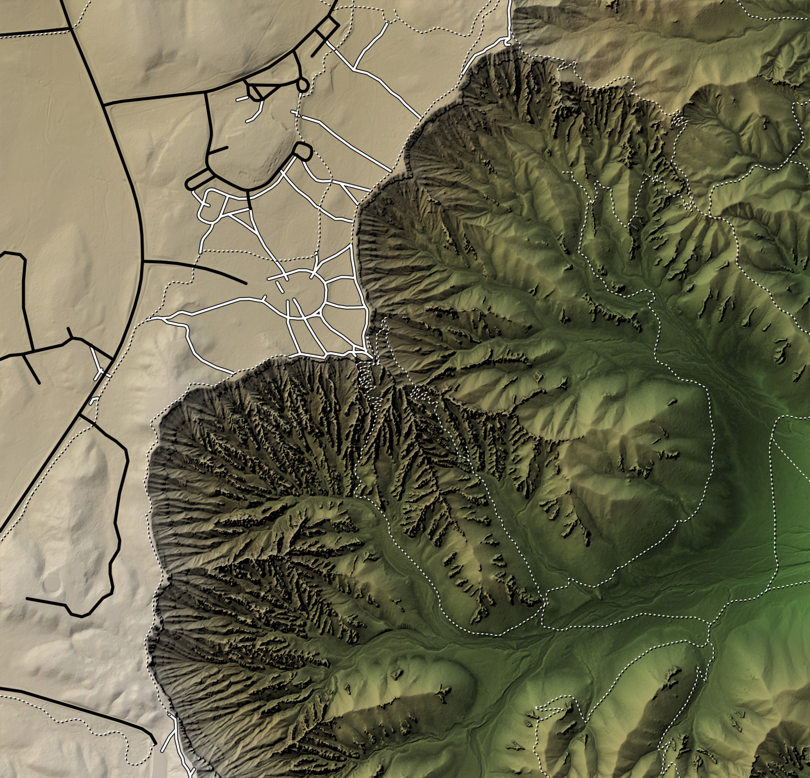
Cool! Let’s save these overlays into their own layer, so we can adjust the base map separately later (if we want to).
trails_layer = generate_line_overlay(bryce_footpaths,extent = extent_zoomed,
                                    linewidth = 10, color="black",
                                    heightmap = bryce_zoom_mat) %>%
  add_overlay(generate_line_overlay(bryce_footpaths,extent = extent_zoomed,
                                    linewidth = 6, color="white",
                                    heightmap = bryce_zoom_mat)) %>%
  add_overlay(generate_line_overlay(bryce_trails,extent = extent_zoomed,
                                    linewidth = 3, color="black", lty=3, offset = c(2,-2),
                                    heightmap = bryce_zoom_mat)) %>%
  add_overlay(generate_line_overlay(bryce_trails,extent = extent_zoomed,
                                    linewidth = 3, color="white", lty=3,
                                    heightmap = bryce_zoom_mat)) %>%
  add_overlay(generate_line_overlay(bryce_roads,extent = extent_zoomed,
                                    linewidth = 8, color="grey30",
                                    heightmap = bryce_zoom_mat))
Now, let’s add some other features. We’ll pull waterways by requesting the waterway feature from OSM. We’ll load the object, reproject it to match our coordinate system, and overlay it in blue underneath our trail layer. There’s not actually many active streams in Bryce—these are intermittent streams, as we see when we print the object below—but it’s a good demonstration on how to add them to our map.
bryce_water_lines = opq(osm_bbox) %>%
  add_osm_feature("waterway") %>%
  osmdata_sf()
bryce_water_line
## Object of class 'osmdata' with:
## $bbox : 37.614998,-112.174228,37.629084,-112.15623
## $overpass_call : The call submitted to the overpass API
## $meta : metadata including timestamp and version numbers
## $osm_points : 'sf' Simple Features Collection with 493 points
## $osm_lines : 'sf' Simple Features Collection with 13 linestrings
## $osm_polygons : 'sf' Simple Features Collection with 0 polygons
## $osm_multilines : NULL
## $osm_multipolygons : NULLbryce_water_lines$osm_line## Simple feature collection with 13 features and 4 fields
## geometry type: LINESTRING
## dimension: XY
## bbox: xmin: -112.1677 ymin: 37.61215 xmax: -112.1374 ymax: 37.63255
## CRS: EPSG:4326
## First 10 features:
## osm_id name intermittent waterway
## 451498495 451498495 Bryce Creek yes stream
## 451498514 451498514 <NA> yes stream
## 451498531 451498531 <NA> yes stream
## 451498543 451498543 <NA> yes stream
## 650406551 650406551 <NA> yes stream
## 650406552 650406552 <NA> yes stream
## 650406554 650406554 <NA> yes stream
## 650406555 650406555 <NA> yes stream
## 650406556 650406556 <NA> yes stream
## 650522440 650522440 <NA> yes stream
## geometry
## 451498495 LINESTRING (-112.1672 37.62...
## 451498514 LINESTRING (-112.1656 37.61...
## 451498531 LINESTRING (-112.1623 37.62...
## 451498543 LINESTRING (-112.16 37.6283...
## 650406551 LINESTRING (-112.1672 37.61...
## 650406552 LINESTRING (-112.1636 37.62...
## 650406554 LINESTRING (-112.1589 37.61...
## 650406555 LINESTRING (-112.1642 37.62...
## 650406556 LINESTRING (-112.1611 37.62...
## 650522440 LINESTRING (-112.1584 37.62...bryce_streams = st_transform(bryce_water_lines$osm_lines,crs=crs(bryce))
stream_layer = generate_line_overlay(bryce_streams,extent = extent_zoomed,
linewidth = 4, color="skyblue2",
heightmap = bryce_zoom_mat)
base_map %>%
add_overlay(stream_layer, alphalayer = 0.8) %>%
add_overlay(trails_layer) %>%
plot_map()
Now let’s add some polygon features. We can pull those out of the parking feature from OSM to get parking lots, building to get buildings, and tourism to get camp grounds and picnic areas. We’ll add these layers before the trails so it doesn’t obscure the trail information.
bryce_parking = opq(osm_bbox) %>%
  add_osm_feature("parking") %>%
  osmdata_sf()

bryce_building = opq(osm_bbox) %>%
  add_osm_feature("building") %>%
  osmdata_sf()

bryce_tourism = opq(osm_bbox) %>%
  add_osm_feature("tourism") %>%
  osmdata_sf()

bryce_parking_poly = st_transform(bryce_parking$osm_polygons,crs=crs(bryce))
bryce_building_poly = st_transform(bryce_building$osm_polygons,crs=crs(bryce))
bryce_tourism_poly = st_transform(bryce_tourism$osm_polygons,crs=crs(bryce))

bryce_sites_poly = bryce_tourism_poly %>%
  filter(tourism %in% c("picnic_site", "camp_site"))

polygon_layer = generate_polygon_overlay(bryce_parking_poly, extent = extent_zoomed,
                                    heightmap = bryce_zoom_mat, palette="grey30") %>%
  add_overlay(generate_polygon_overlay(bryce_building_poly, extent = extent_zoomed,
                                    heightmap = bryce_zoom_mat, palette="darkred")) %>%
  add_overlay(generate_polygon_overlay(bryce_sites_poly, extent = extent_zoomed,
                                    heightmap = bryce_zoom_mat, palette="darkgreen"), alphalayer = 0.6)

base_map %>%
  add_overlay(polygon_layer) %>%
  add_overlay(stream_layer, alphalayer = 0.8) %>%
  add_overlay(trails_layer) %>%
  plot_map()
This is pretty, but we need context! Let’s add some of the natural features in the landscape as labels, using generate_label_overlay().
bryce_tourism_points = st_transform(bryce_tourism$osm_points,crs=crs(bryce))

bryce_attractions = bryce_tourism_points %>%
  filter(tourism == "attraction")

base_map %>%
  add_overlay(polygon_layer) %>%
  add_overlay(stream_layer, alphalayer = 0.8) %>%
  add_overlay(trails_layer) %>%
  add_overlay(generate_label_overlay(bryce_attractions, extent = extent_zoomed,
                                     text_size = 2, point_size = 1,
                                     seed=1,
                                     heightmap = bryce_zoom_mat, data_label_column = "name")) %>%
  plot_map()
Wait—where are the labels? They’re there, if you look hard enough. One of the difficulties you encounter adding labels to maps is obtaining sufficient contrast between the text and underlying map: dark labels on a dark, changing background are hard to read. Light labels on light areas present the same problem. A fairly standard solution to this problem is to add a “halo” of a different color to your text—it ensures your text will always be readable, regardless of the background. Let’s do that using the built-in halo arguments: setting halo_color to a color activates the halo.
base_map %>%
  add_overlay(polygon_layer) %>%
  add_overlay(stream_layer, alphalayer = 0.8) %>%
  add_overlay(trails_layer) %>%
  add_overlay(generate_label_overlay(bryce_attractions, extent = extent_zoomed,
                                     text_size = 2, point_size = 1,
                                     halo_color = "white",halo_expand = 5,
                                     seed=1,
                                     heightmap = bryce_zoom_mat, data_label_column = "name")) %>%
  plot_map()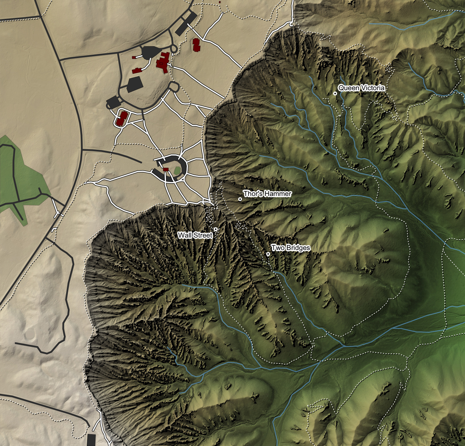
If you don’t like the solid border, you can blur the halo layer a bit for a softer outline. We’ll also make the halo slightly transparent all the way through by setting the halo_alpha argument.
base_map %>%
  add_overlay(polygon_layer) %>%
  add_overlay(stream_layer, alphalayer = 0.8) %>%
  add_overlay(trails_layer) %>%
  add_overlay(generate_label_overlay(bryce_attractions, extent = extent_zoomed,
                                     text_size = 2, point_size = 1, color = "black",
                                     halo_color = "white", halo_expand = 10,
                                     halo_blur = 20, halo_alpha = 0.8,
                                     seed=1,
                                     heightmap = bryce_zoom_mat, data_label_column = "name")) %>%
  plot_map()
The appearance of the halo is a bit jarring over the dark background—let’s swap the color palette so the halo isn’t so noticeable.
base_map %>%
  add_overlay(polygon_layer) %>%
  add_overlay(stream_layer, alphalayer = 0.8) %>%
  add_overlay(trails_layer) %>%
  add_overlay(generate_label_overlay(bryce_attractions, extent = extent_zoomed,
                                     text_size = 2, point_size = 2, color = "white",
                                     halo_color = "black", halo_expand = 10,
                                     halo_blur = 20, halo_alpha = 0.8,
                                     seed=1,
                                     heightmap = bryce_zoom_mat, data_label_column = "name")) %>%
  plot_map()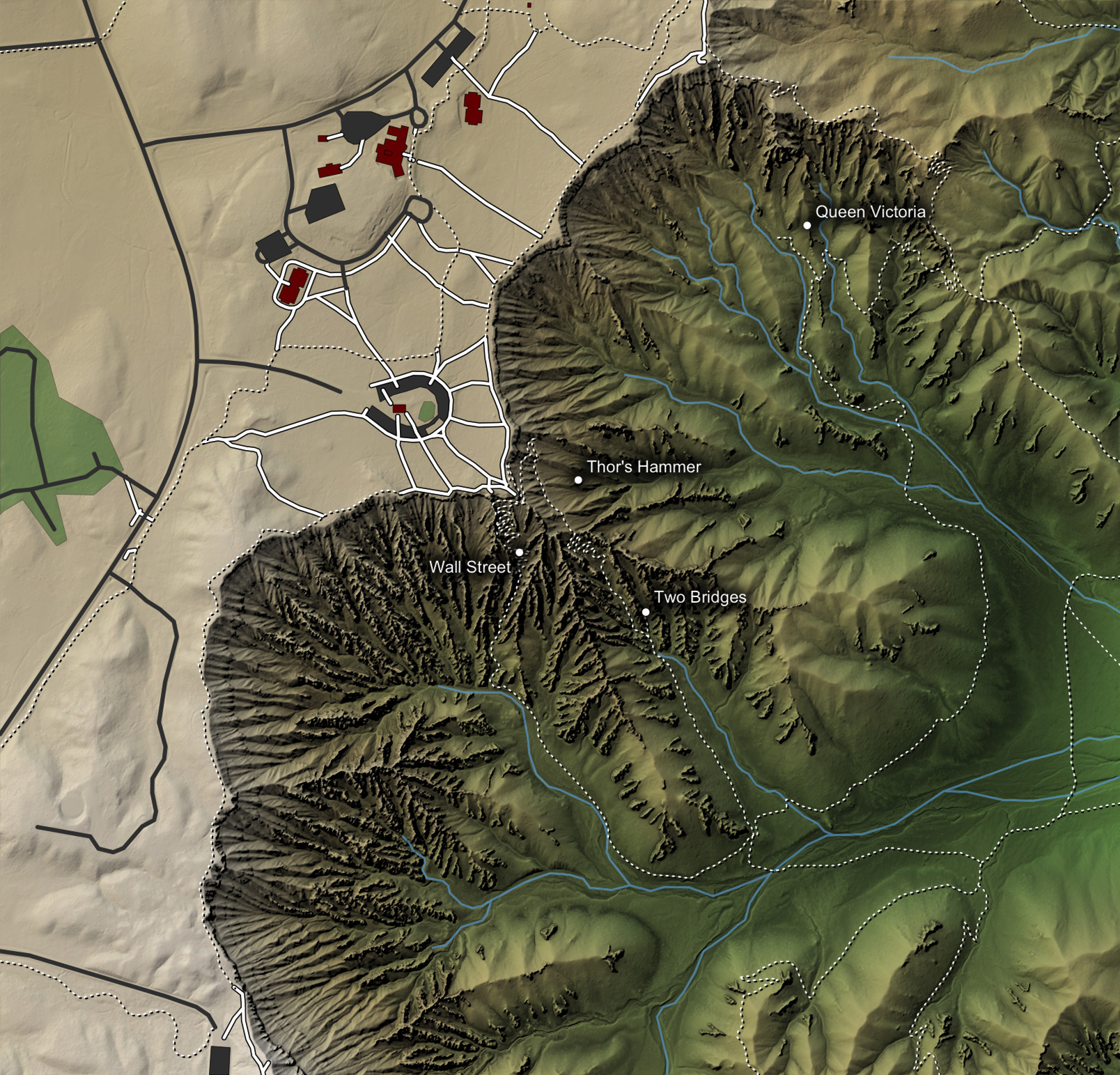
Looks good! Our text now seamlessly blends into our map, but the background doesn’t interfere with the text’s legibility. Now, to finish the map: let’s add a title.
base_map %>%
  add_overlay(polygon_layer) %>%
  add_overlay(stream_layer, alphalayer = 0.8) %>%
  add_overlay(trails_layer) %>%
  add_overlay(generate_label_overlay(bryce_attractions, extent = extent_zoomed,
                                     text_size = 2, point_size = 2, color = "white",
                                     halo_color = "black", halo_expand = 10,
                                     halo_blur = 20, halo_alpha = 0.8,
                                     seed=1, heightmap = bryce_zoom_mat, data_label_column = "name")) %>%
  plot_map(title_text = "Bryce Canyon National Park, Utah", title_offset = c(15,15),
           title_bar_color = "grey5", title_color = "white", title_bar_alpha = 1)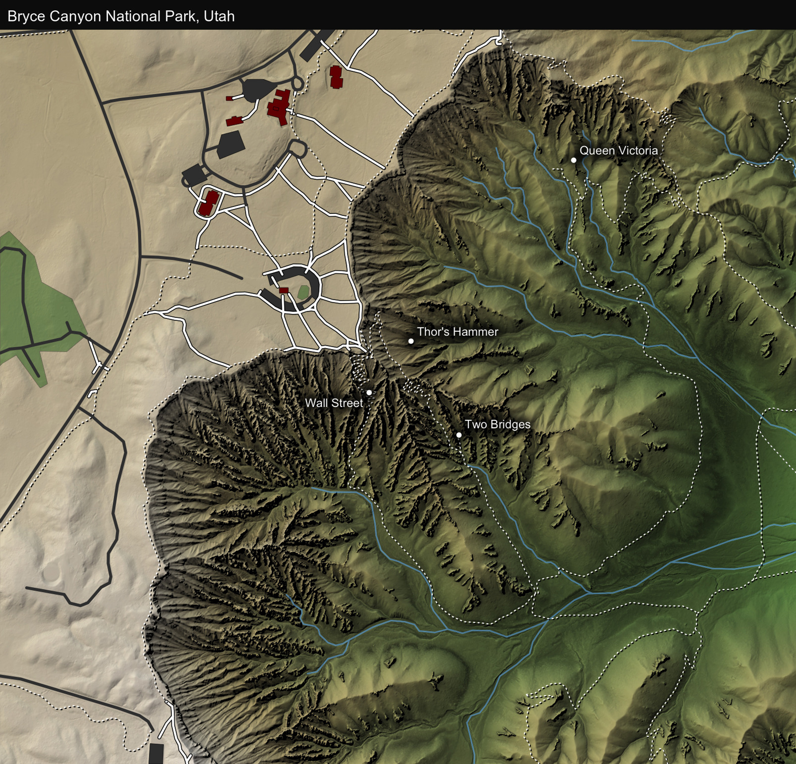
Rayshader also makes it easy to visualize this map in 3D.
base_map %>%
  add_overlay(polygon_layer) %>%
  add_overlay(stream_layer, alphalayer = 0.8) %>%
  add_overlay(trails_layer) %>%
  plot_3d(bryce_zoom_mat, windowsize=c(1200,800))
render_camera(theta=240,  phi=30, zoom=0.3,  fov=60)
render_snapshot()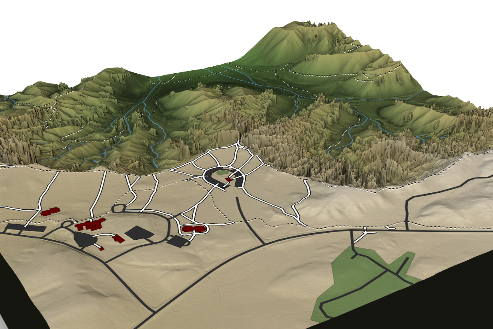
And now you know how to add Open Street Map data to your map in R! Feed free to copy this code and try it yourself. Of course, you might not want to copy this map exactly for your region—it sure would be nice to know how easy it is to restyle your map to your tastes!
😁👇
Restyling Your Map
The great thing about working in a programming language is how easy it is to completely revamp the appearance with the map just by changing a few lines of code—no manual work required! Here are a few examples of re-styling this map in rayshader:
Let’s generate a new base map with a better shading method for a 3D map (lamb_shade() darkens the steep slopes too much in 3D). An ambient_shade() layer will provide much softer shadows in those regions, as it models diffuse light (rather than direct lighting).
#Exaggerate surface 5x for darker ambient occlusion shadows
amb_layer = ambient_shade(bryce_zoom_mat,zscale=1/5)

bryce_zoom_mat %>%
  height_shade() %>%
  add_shadow(texture_shade(bryce_zoom_mat,detail=8/10,contrast=9,brightness = 11), 0) %>%
  add_shadow(amb_layer,0) %>%
  add_overlay(polygon_layer) %>%
  add_overlay(stream_layer, alphalayer = 0.8) %>%
  add_overlay(trails_layer) %>%
  plot_3d(bryce_zoom_mat, windowsize = c(1200,1200), theta=40,  phi=50, zoom=0.4,  fov=90)

render_snapshot()
rgl::rgl.close()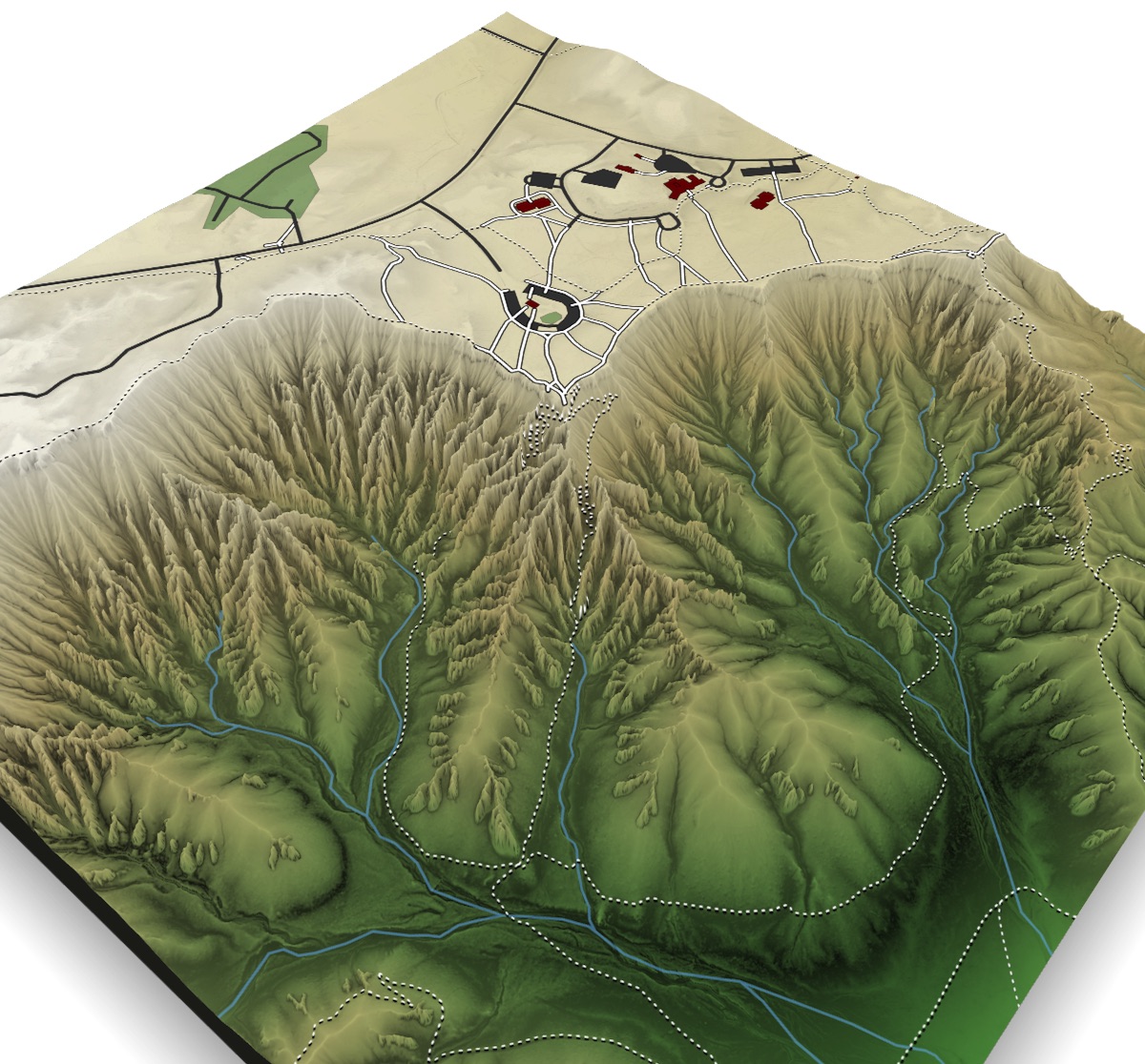
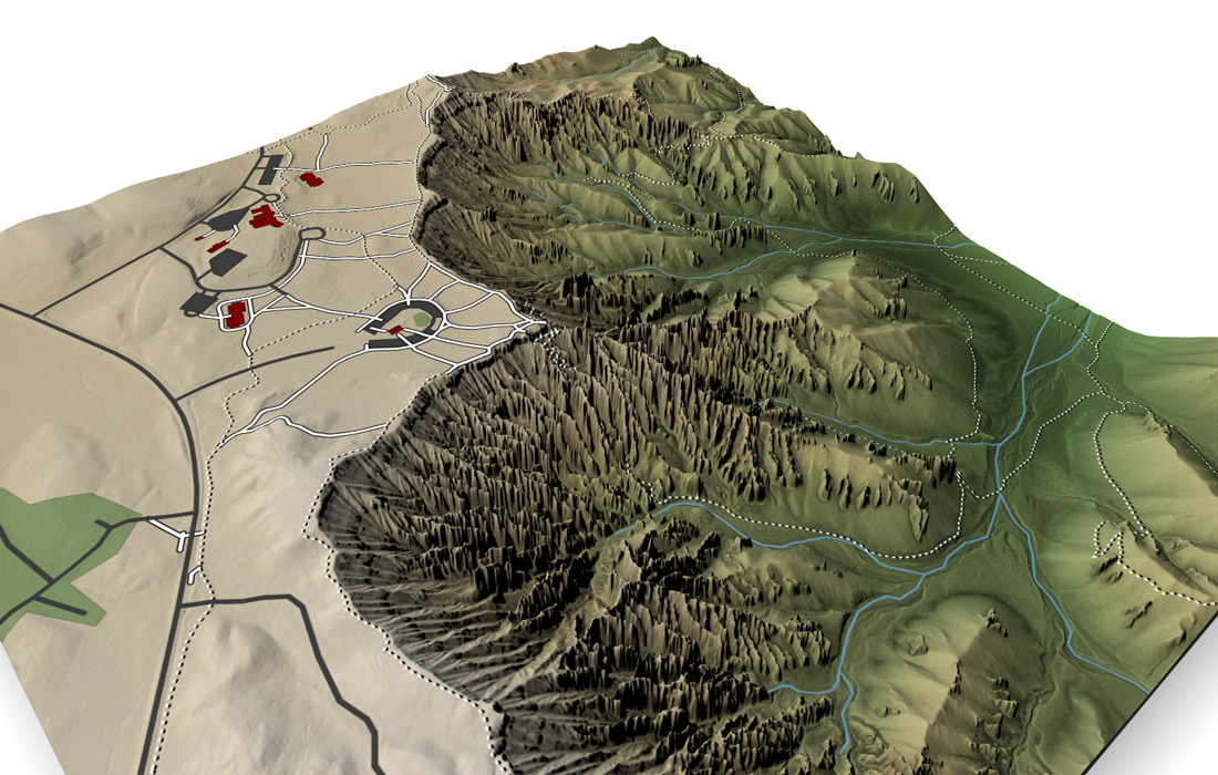
Compare the edges of the steep valleys in this 3D version to the rotating map at the top of this post—unlike that one, these slopes aren’t black.
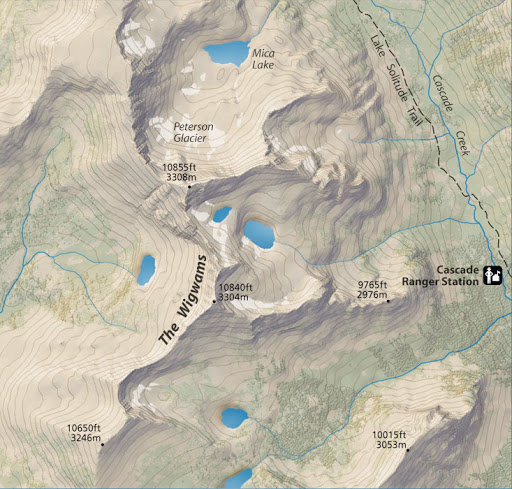
Now, let’s create a faux National Park Service map. Here’s an example of the style:
Here, I change up the height_shade() color ramp and water color, add a pure white overlay to lighten the entire map (which makes the trails pop from the background), change to black labels with a soft white outline, add dense semi-transparent light-brown contours at 5 meter intervals, and add a black title bar (which is standard for NPS maps). The only thing missing here is NPS symbology.
watercolor = "#2a89b3"
maxcolor = "#e6dbc8"
mincolor = "#b6bba5"
contour_color = "#7d4911"

bryce_zoom_mat %>%
  height_shade(texture = grDevices::colorRampPalette(c(mincolor,maxcolor))(256)) %>%
  add_shadow(lamb_shade(bryce_zoom_mat),0.2) %>%
  add_overlay(generate_contour_overlay(bryce_zoom_mat, color = contour_color,
                                       linewidth = 2, levels=seq(min(bryce_zoom_mat), max(bryce_zoom_mat), by=5)),alphalayer = 0.5) %>%
  add_overlay(polygon_layer) %>%
  add_overlay(height_shade(bryce_zoom_mat,texture = "white"), alphalayer=0.2) %>%
  add_overlay(generate_line_overlay(bryce_streams,extent = extent_zoomed,
                                    linewidth = 4, color=watercolor,
                                    heightmap = bryce_zoom_mat)) %>%
  add_overlay(generate_line_overlay(bryce_footpaths,extent = extent_zoomed,
                                    linewidth = 4, color="black",
                                    heightmap = bryce_zoom_mat)) %>%
  add_overlay(generate_line_overlay(bryce_trails,extent = extent_zoomed,
                                    linewidth = 4, color="black", lty=2,
                                    heightmap = bryce_zoom_mat)) %>%
  add_overlay(generate_line_overlay(bryce_roads,extent = extent_zoomed,
                                    linewidth = 12, color="black",
                                    heightmap = bryce_zoom_mat)) %>%
  add_overlay(generate_line_overlay(bryce_roads,extent = extent_zoomed,
                                    linewidth = 8, color="white",
                                    heightmap = bryce_zoom_mat)) %>%
  add_overlay(generate_label_overlay(bryce_attractions, extent = extent_zoomed,
                                     text_size = 2, point_size = 2, color = "black",
                                     halo_color = "#e6e1db", halo_expand = 5,
                                     halo_blur = 2, halo_alpha = 0.8,
                                     seed=1, heightmap = bryce_zoom_mat,
                                     data_label_column = "name")) %>%
  plot_map(title_text="Bryce Canyon National Park, Utah", title_color = "white",
           title_bar_alpha = 1, title_bar_color = "black")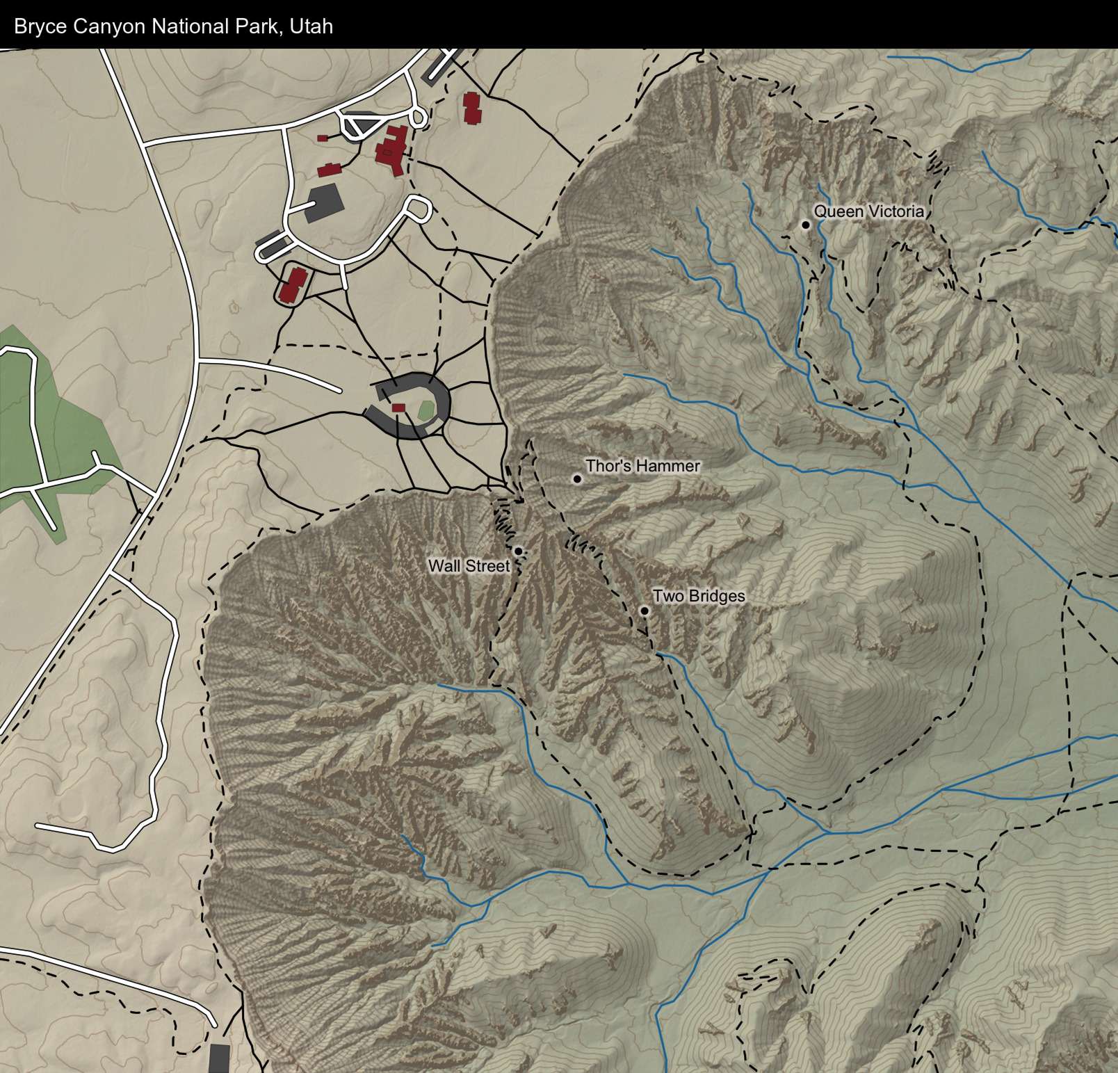
Let’s look at an animated version of what that looks like, built-up layer-by-layer.
What if we want a map that’s more informational? Let’s create a trail map for the area. We’ll extract the individual trails to color them separately, and place labels down adjacent to a point along the trail. We’ll also remove all other color from the map and lighten the underlying map to make the trails the focal point. To further differentiate the trail labels from the location labels, we’ll make the trail font bold by setting font = 2 and giving them a white outline.
navajo_trail = bryce_trails %>%
  filter(name == "Navajo Loop Trail")

rim_trail = bryce_trails %>%
  filter(name == "Rim Trail")

queen_trail = bryce_trails %>%
  filter(name %in% c("Queen's Garden", "Queen's Garden Trail"))

navajo_coords = st_coordinates(navajo_trail)
rim_coords = st_coordinates(rim_trail)
queen_coords = st_coordinates(queen_trail)

label_navajo_coord = navajo_coords[34,1:2]
label_rim_coord = rim_coords[50,1:2]
label_queen_coord = queen_coords[35,1:2]


bryce_zoom_mat %>%
  height_shade(texture = "white") %>%
  add_shadow(lamb_shade(bryce_zoom_mat),0.6) %>%
  add_overlay(generate_contour_overlay(bryce_zoom_mat, color = "black",
                                       linewidth = 2, levels=seq(min(bryce_zoom_mat),
                                       max(bryce_zoom_mat), by=5)),alphalayer = 0.2) %>%
  add_overlay(generate_polygon_overlay(bryce_building_poly, extent = extent_zoomed,
                                    heightmap = bryce_zoom_mat, palette="black")) %>%
  add_overlay(generate_polygon_overlay(bryce_parking_poly, extent = extent_zoomed,
                                    heightmap = bryce_zoom_mat, palette="grey30")) %>%
  add_overlay(generate_line_overlay(bryce_footpaths,extent = extent_zoomed,
                                    linewidth = 4, color="grey30",
                                    heightmap = bryce_zoom_mat)) %>%
  add_overlay(generate_line_overlay(bryce_roads,extent = extent_zoomed,
                                    linewidth = 8, color="grey30",
                                    heightmap = bryce_zoom_mat)) %>%
  add_overlay(generate_line_overlay(navajo_trail,extent = extent_zoomed,
                                    linewidth = 6, color="red",
                                    heightmap = bryce_zoom_mat)) %>%
  add_overlay(generate_line_overlay(queen_trail,extent = extent_zoomed,
                                    linewidth = 6, color="orange",
                                    heightmap = bryce_zoom_mat)) %>%
  add_overlay(generate_line_overlay(rim_trail,extent = extent_zoomed,
                                    linewidth = 6, color="purple",
                                    heightmap = bryce_zoom_mat)) %>%
  add_overlay(generate_label_overlay(bryce_attractions, extent = extent_zoomed,
                                     text_size = 2, point_size = 2, color = "black",
                                     seed=1, heightmap = bryce_zoom_mat,
                                     data_label_column = "name")) %>%
  add_overlay(generate_label_overlay(label = "Navajo Loop Trail",
                                     x=label_navajo_coord[1]-30, y=label_navajo_coord[2],
                                     extent = extent_zoomed, text_size = 3, color = "red", font=2,
                                     halo_color = "white", halo_expand = 4, point_size = 0,
                                     seed=1, heightmap = bryce_zoom_mat)) %>%
  add_overlay(generate_label_overlay(label = "Rim Trail",
                                     x=label_rim_coord[1]+200, y=label_rim_coord[2],
                                     extent = extent_zoomed, text_size = 3, color = "purple", font=2,
                                     halo_color = "white", halo_expand = 4, point_size = 0,
                                     seed=1, heightmap = bryce_zoom_mat)) %>%
  add_overlay(generate_label_overlay(label = "Queen's Garden Trail",
                                     x=label_queen_coord[1], y=label_queen_coord[2],
                                     extent = extent_zoomed, text_size = 3, color = "orange", font=2,
                                     halo_color = "white", halo_expand = 4, point_size = 0,
                                     seed=1, heightmap = bryce_zoom_mat)) %>%
  plot_map(title_text="Bryce Canyon National Park Trails, Sunset Point", title_color = "white",
           title_bar_alpha = 1, title_bar_color = "black")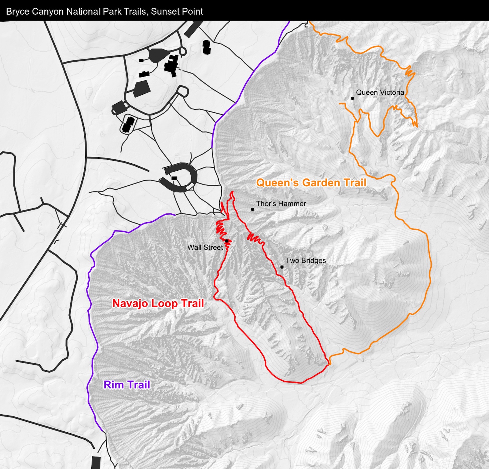
Finally, let’s create a map in the style of the great Swiss cartographer, Eduard Imhof. He had a particular style well-represented by the sphere_shade() function (see this blog post for examples). Here’s an example of his style:
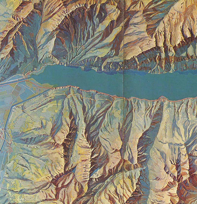
We can switch up our color palette in sphere_shade() to create a facsimile of Eduard’s work. We’ll also remove the contours and use the generate_altitude_overlay() function to create an atmospheric scattering effect by generating a bluish tint at lower elevations. This is a technique cartographers use to help you distinguish between high elevations and lower elevations without resorting to contours or 3D.
bryce_zoom_mat %>%
  sphere_shade(texture = create_texture("#f5dfca","#63372c","#dfa283","#195f67","#c2d1cf",
                                        cornercolors = c("#ffc500", "#387642", "#d27441","#296176")),
               sunangle = 0, colorintensity = 5) %>%
  add_shadow(lamb_shade(bryce_zoom_mat),0.2) %>%
  add_overlay(generate_altitude_overlay(height_shade(bryce_zoom_mat, texture = "#91aaba"),
                                        bryce_zoom_mat,
                                        start_transition = min(bryce_zoom_mat)-200,
                                        end_transition = max(bryce_zoom_mat))) %>%
  add_overlay(generate_line_overlay(bryce_footpaths,extent = extent_zoomed,
                                    linewidth = 7, color="black",
                                    heightmap = bryce_zoom_mat),alphalayer = 0.8) %>%
  add_overlay(generate_line_overlay(bryce_trails,extent = extent_zoomed,
                                    linewidth = 6, color="black",
                                    heightmap = bryce_zoom_mat),alphalayer = 0.8) %>%
  add_overlay(generate_line_overlay(bryce_roads,extent = extent_zoomed,
                                    linewidth = 8, color="black",
                                    heightmap = bryce_zoom_mat),alphalayer = 0.8) %>%
  add_overlay(generate_line_overlay(bryce_footpaths,extent = extent_zoomed,
                                    linewidth = 4, color="white",
                                    heightmap = bryce_zoom_mat),alphalayer = 0.8) %>%
  add_overlay(generate_line_overlay(bryce_trails,extent = extent_zoomed,
                                    linewidth = 3, color="white",
                                    heightmap = bryce_zoom_mat),alphalayer = 0.8) %>%
  add_overlay(generate_line_overlay(bryce_roads,extent = extent_zoomed,
                                    linewidth = 5, color="white",
                                    heightmap = bryce_zoom_mat),alphalayer = 0.8) %>%
  add_overlay(generate_polygon_overlay(bryce_building_poly, extent = extent_zoomed,
                                    heightmap = bryce_zoom_mat, palette="#292b26"),
              alphalayer = 0.8) %>%
  plot_map()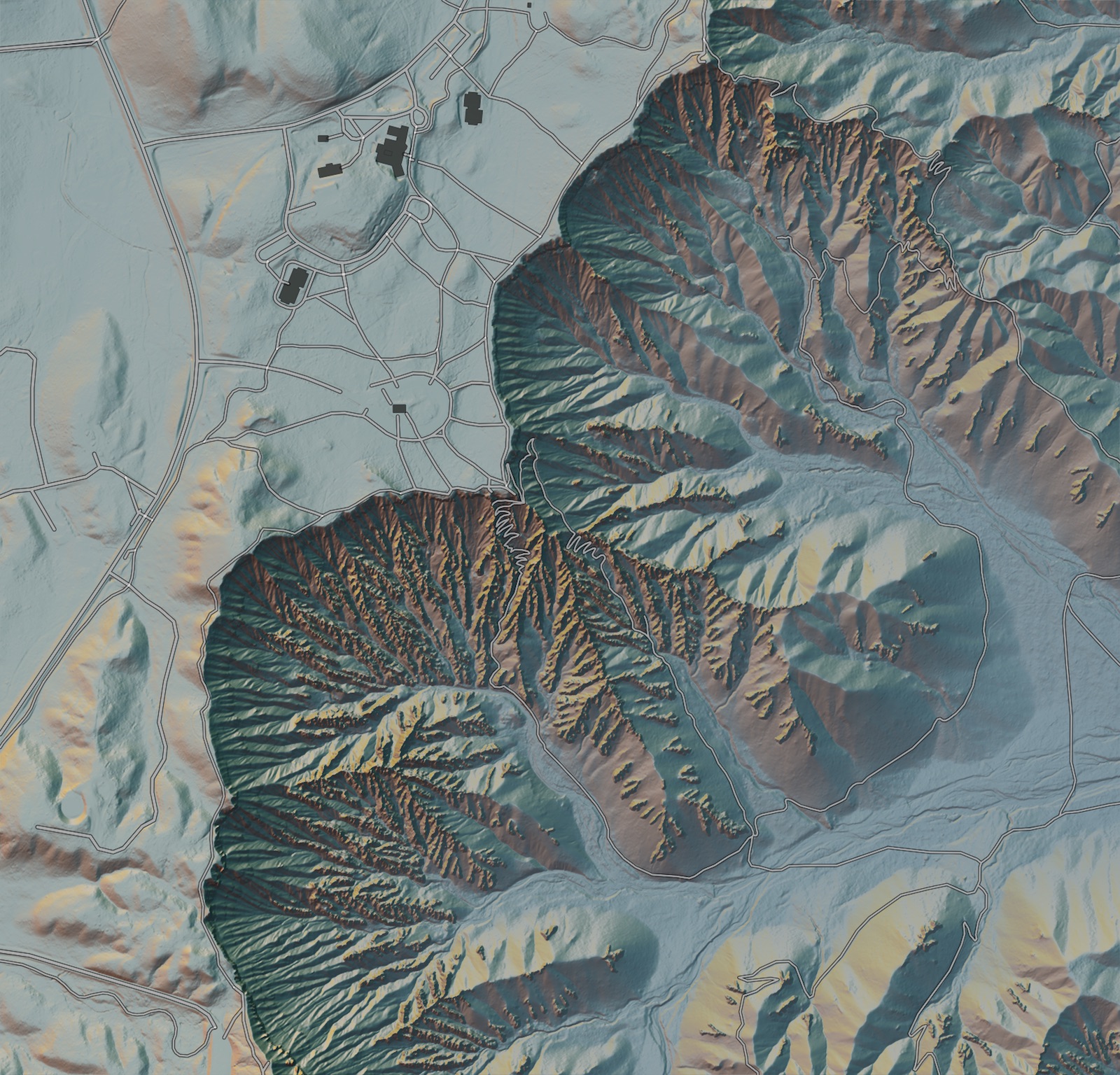
And here’s an animated flipbook building this map:
And that ends my tutorial! I hope it’s now clear how easy it is to add Open Street Map data to your rayshader maps, and how simple it is to customize the style and appearance of your map using nothing but code. If you create a fun or interesting visualization with rayshader, be sure to post it to Twitter with the hashtags #rstats and #rayshader. Happy mapping!