DataCoaster Tycoon: Building 3D Rollercoaster Tours of Your Data in R
3D data visualization presents unique challenges for the data viz practitioner. In 2D, you have to tackle problems like “How do I adjust the inner margins?” or “How can I nudge these overlapping labels away from each other?” or “Uhh… how do I do remove the legend again?” Formidable mainly because you need to know the correct code incantations to get the spacing/style you want, but conceptually not that dissimilar from fighting with Microsoft Word to properly layout a document or cutting and pasting together a tri-fold science fair project.
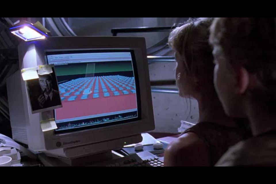
3D data visualizations, on the other hand, require an entirely different set of skills: rather than laying out points and lines on a flat 2D surface, you’re now required to embed your data in an abstract 3D space, set up camera angles and focal points, generate proper lighting, deal with data physically obscuring other data, set up your axes in 3D space, and more. The extra dimension provides additional freedoms but makes creating even simple plots fairly complex. And this complexity only increases when you actually want to generate an animation that travels through the space: suddenly, you now have to deal with animating your camera orientation AND position, and do it in a way that doesn’t make your audience nauseous. And most people aren’t great with navigating a 3D space to begin with (which is why we don’t all navigate our computers like we’re hacking Unix in Jurassic Park), much less setting up complex animations in that space via code.
What does any of this have to do with rollercoasters? Well, for a while I’ve been working on an animation interface for my R rendering package, rayrender. This interface takes a series of user-provided key frames of camera positions and orientations in 3D space and generates a smooth continuous camera track between them. However, many people have a hard enough time conceptualizing tweening between key frames in 2D: How do I create an easy-to-understand example of transitioning between 6D states (3D position + 3D orientation)? What’s a relatable example of smoothly moving through a 3D space along a well-defined track?
… Rollercoasters!
So this post isn’t about of a new type of 3D visualizations (Coasterplots!), but is rather a tech demonstration showing how to create animations through 3D space with R and rayrender’s new camera animation API. The rollercoaster part is because it’s a fun example, but slow down the coaster and add some narration and you have a guided monorail tour through your data—a concept that I think has real value. But for now, let’s just stick with the thrill rides to have some fun and show off what rayrender can do. Let’s get started!
The key new features in rayrender are the generate_camera_motion() and render_animation() functions, which work together to generate frames of an animation. generate_camera_motion() takes your key positions and number of frames, and generates the steps between those frames for a smooth camera transition. The default is to connect the key frames with cubic Bézier curves, and the implementation ensures continuity of the camera’s motion position and derivative. Rather than specifying an orientation with Euler angles (which have issues of gimble lock and aren’t very user-friendly), the orientation is animated via a lookat position. There are other camera properties you can animate (field of view, focal length, orientation, aperture), but we’re just going to stick with the basics for this demo. You can also specify different tween types instead of Bézier curves: linear, quadratic, cubic, and exponential transitions are also supported. Here’s an example from my twitter page of animating between key frames with cubic transitions:
Who needs fancy paid GIS suites or complex renderers with byzantine user interfaces? Fly through your data with #rstats + #rayshader + #rayrender! pic.twitter.com/D8deNogxUt
— Tyler Morgan-Wall (@tylermorganwall) April 6, 2020
render_animation() takes your rayrender scene along with the data frame of camera data provided by generate_camera_motion() and generates the frames of your animation. This is far more efficient than repeated calls to render_scene(), as the acceleration structure used by rayrender for ray intersection doesn’t need to be rebuilt for every frame. For large scenes, this can be a non-trivial amount of time saved per frame—sometimes equal to the rendering time itself. The images are saved to disk and you can restart the animation from any frame, which allows you to interrupt the process without losing all your work.
We’ll start by using rayshader to generate a 3D ggplot of the diamonds dataset. Make sure you have the latest version of rayrender installed.
library(ggplot2)
remotes::install_github("tylermorganwall/rayrender")
library(rayrender)
library(rayshader)

ggdiamonds = ggplot(diamonds, aes(x, depth)) +
  stat_density_2d(aes(fill = stat(nlevel)), geom = "polygon", n = 200, bins = 100,contour = TRUE) +
  facet_wrap(clarity~.) +
  scale_fill_viridis_c(option = "A")
ggdiamond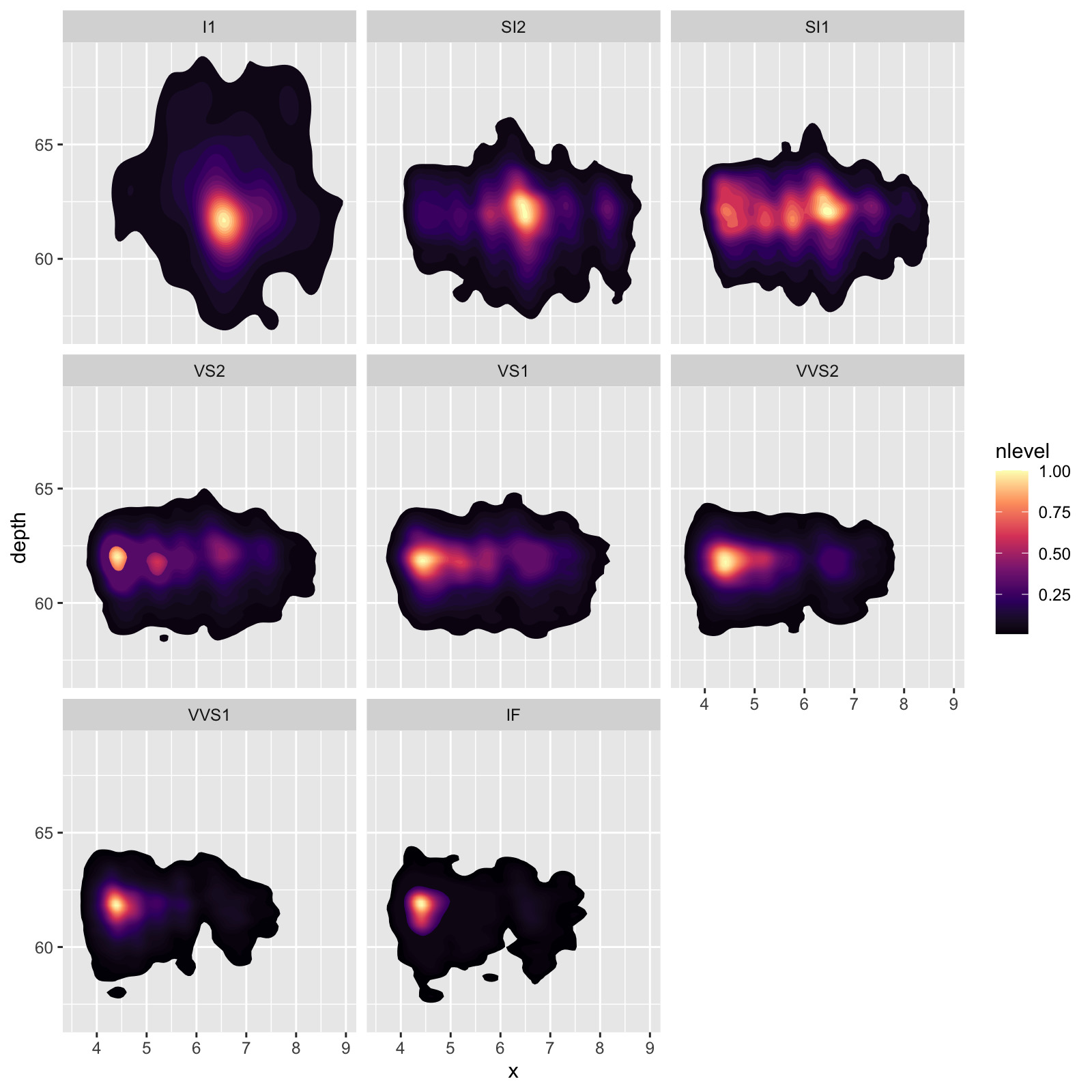
If you’ve never used rayshader, making this density plot 3D is an incredibly easy process (see this blog post for more examples).
plot_gg(ggdiamonds,width=7,height=7,scale=250,windowsize=c(1100,700),
        raytrace=FALSE, zoom = 0.55, phi = 30, triangulate = TRUE, max_error = 0)
render_snapshot()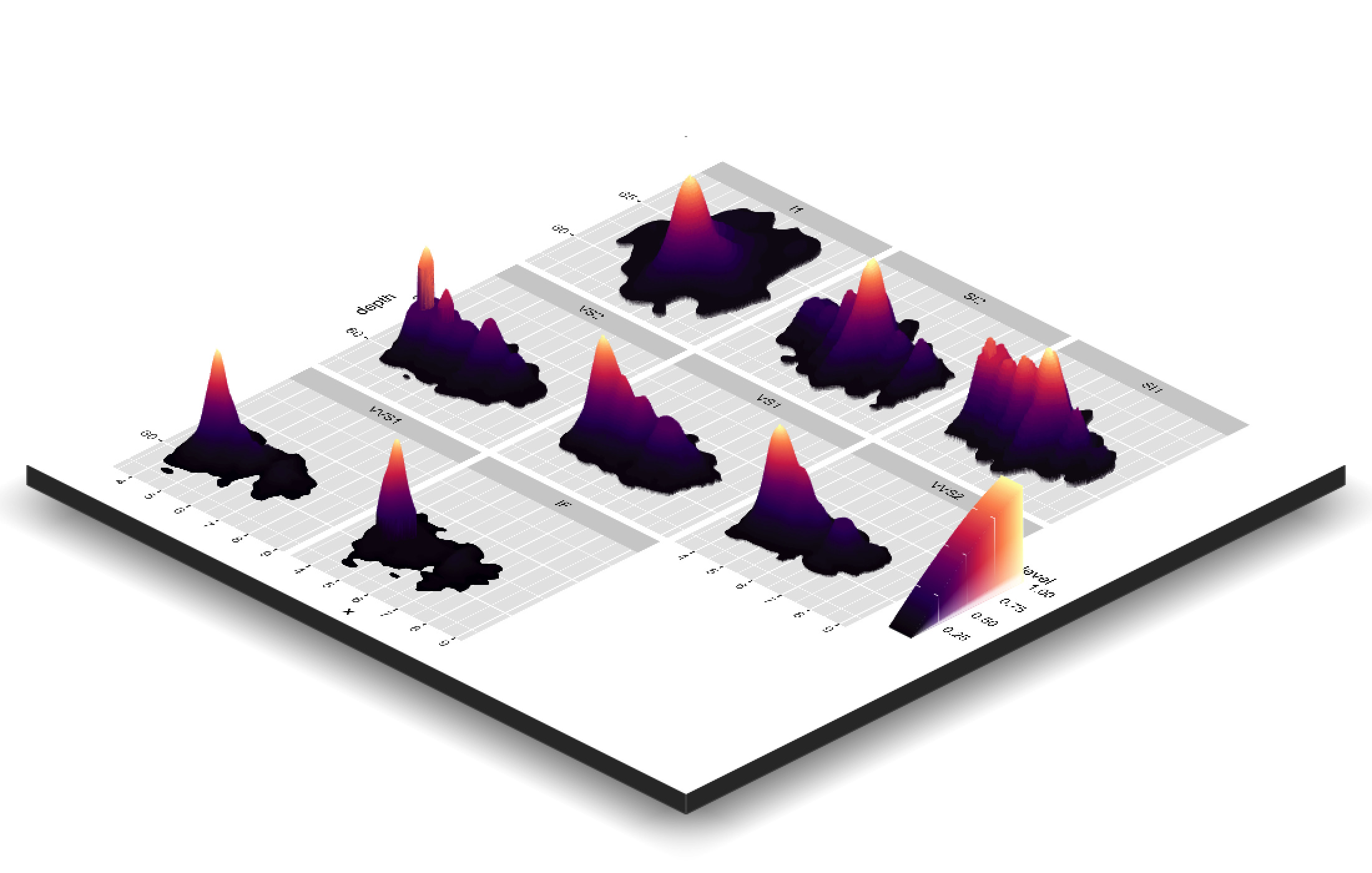
We’ll save an OBJ file to disk so we can load the model into rayrender:
save_obj("ggplot.obj")
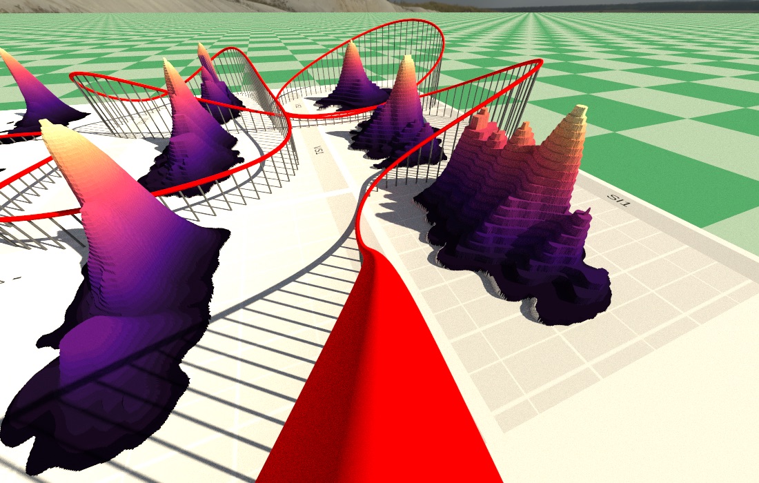
rgl::rgl.close()Let’s see what this looks like in rayrender in an orthographic view (scaled down by a factor of 100 purely for visualization purposes):
disk(radius=1000,y=-1,
     material=diffuse(checkerperiod = 6,checkercolor="#0d401b", color="#496651")) %>%
  add_object(obj_model("ggplot.obj", y=-0.02, texture=TRUE, scale_obj = 1/100)) %>%
  add_object(sphere(y=30,z=10,radius=5,material = light(intensity=40))) %>%
  render_scene(lookfrom=c(20,20,20),fov=0,ortho_dimensions=c(30,30), width=800,height=800)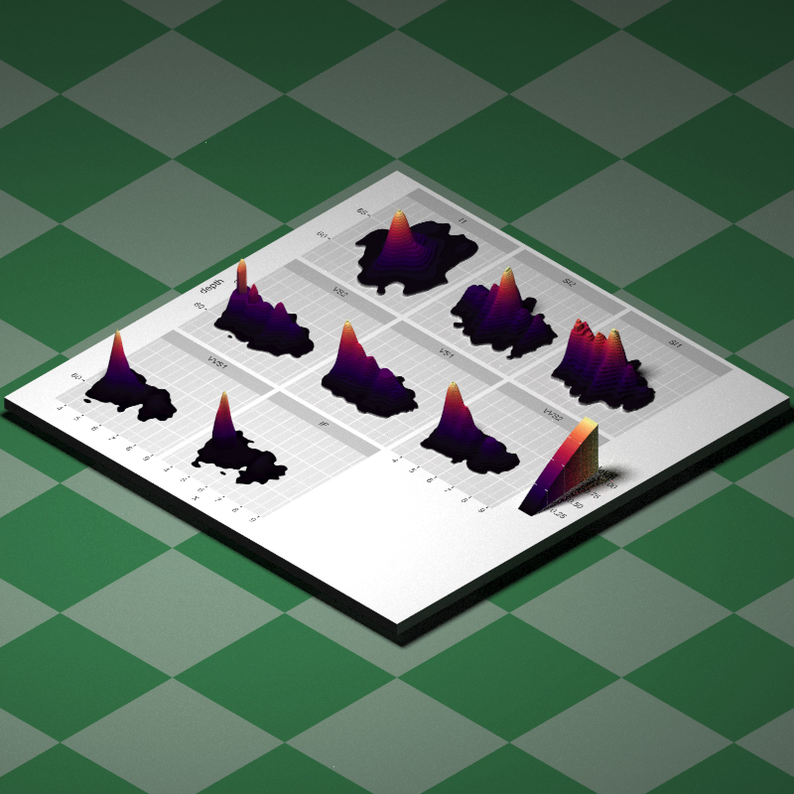
Now, we want to specify a series of points we want to visit around this plot in our rollercoaster. How do we do that in a reasonably user-friendly way? It would be nice to be able to simply click on the areas of the plot we want to visit in order, rather than trying to figure out where they are in our 3D plot. And that’s actually entirely possible in R using the locator() function, which allows you to click on the plot and returns the coordinates of the selected points. Let’s plot the surface texture (saved as raysurface.png during the save_obj() call) in our R device using the rayimage package. We’ll then call the locator() function with our number of desired key frames, and click on the points (in order) we want our rollercoaster to travel through. We then need to scale this from viewpoint coordinates (which are specified in pixels) into our 3D plot, centered at the origin (and flipping the z-coordinates to account for some R-isms).
library(rayimage)
library(raster)
plot_image("raysurface.png")
vals = locator(n=20)
vals$z = vals$y
vals$y = rep(5,length(vals$y))
selected_points = do.call(cbind,vals)
selected_point
## x y z
## [1,] 1923.03521 5 137.8239
## [2,] 1931.48592 5 843.4577
## [3,] 1923.03521 5 1227.9648
## [4,] 1551.20423 5 1363.1761
## [5,] 1289.23239 5 1515.2887
## [6,] 1276.55634 5 1916.6972
## [7,] 799.09155 5 1967.4014
## [8,] 655.42958 5 1380.0775
## [9,] 258.24648 5 1418.1056
## [10,] 215.99296 5 1992.7535
## [11,] 659.65493 5 2018.1056
## [12,] 744.16197 5 1435.0070
## [13,] 625.85211 5 737.8239
## [14,] 279.37324 5 750.5000
## [15,] 85.00704 5 1105.4296
## [16,] 718.80986 5 1265.9930
## [17,] 1234.30282 5 1232.1901
## [18,] 1213.17606 5 708.2465
## [19,] 663.88028 5 615.2887
## [20,] 676.55634 5 108.2465loaded_texture = png::readPNG("raysurface.png")
dim(loaded_texture)## [1] 2100 2100 4#Center at origin, flip, and scale by 1/100 to match our rayrender model
selected_points[,1] = (selected_points[,1] - 2100/2)/100
selected_points[,3] = -(selected_points[,3] - 2100/2)/100
Now let’s plot it on top of the rayrender model to see what it looks like. We ensure the path is closed by setting closed = TRUE in the path() function. We’ll also generate some spheres to place at the key frames to mark their positions.
keylist = list()
for(i in 1:nrow(selected_points)) {
  keylist[[i]] = sphere(x=selected_points[i,1],
                        y=selected_points[i,2],
                        z=selected_points[i,3],radius=0.3,
                        material=diffuse(color="purple"))
}
keyscene = do.call(rbind,keylist)

disk(radius=1000,y=-1,
     material=diffuse(checkerperiod = 6,checkercolor="#0d401b", color="#496651")) %>%
  add_object(obj_model("ggplot.obj", y=-0.02, texture=TRUE, scale_obj = 1/100)) %>%
  add_object(sphere(y=30,z=-10,radius=5,material = light(intensity=40))) %>%
  add_object(path(points=selected_points,width=0.1, closed = TRUE,
                  material=diffuse(color="red"))) %>%
  add_object(keyscene) %>%
  render_scene(lookfrom = c(0, 10, 0), fov = 0, ortho_dimensions = c(30, 30), camera_up = c(0, 0, -1),
               width = 800, height = 800, samples = 256)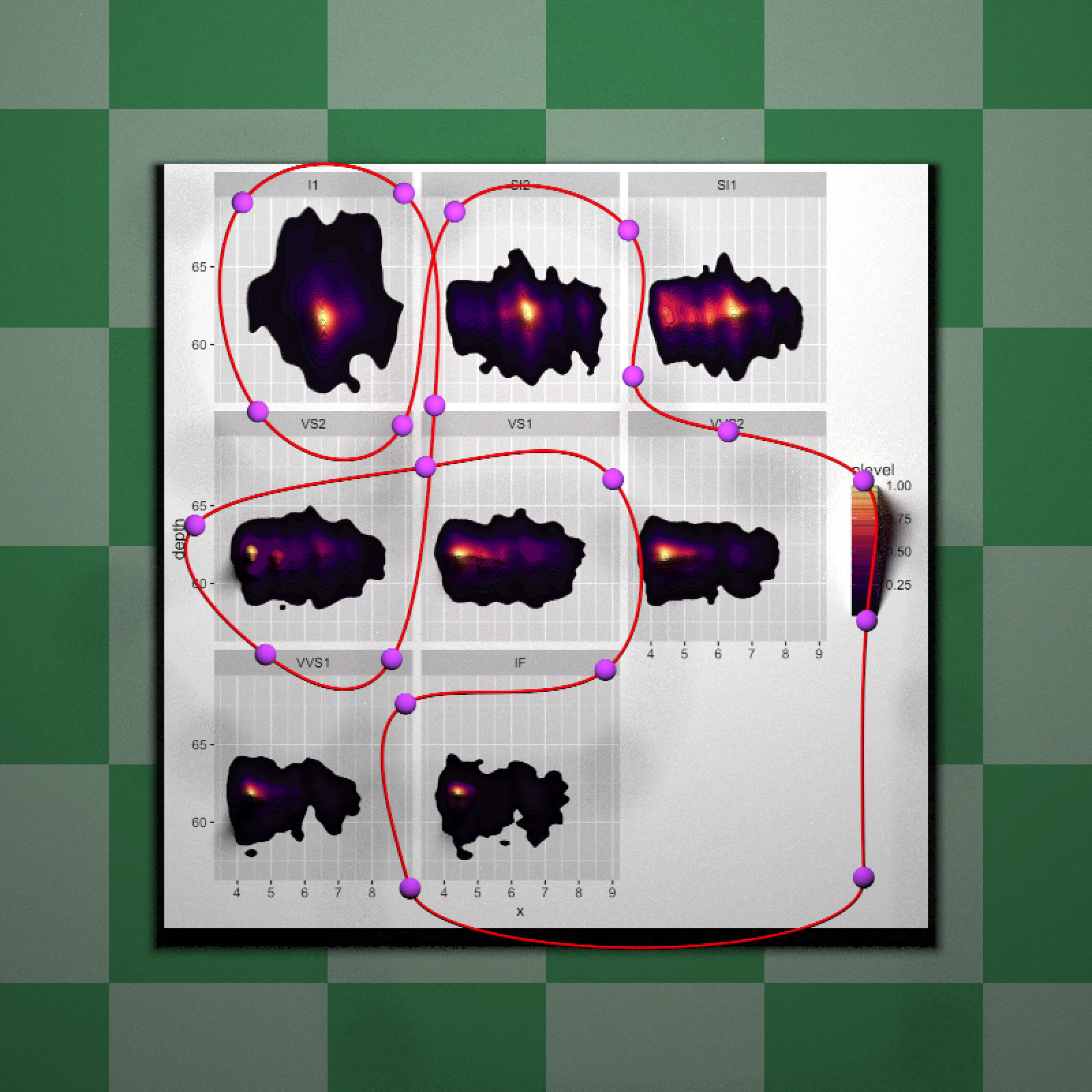
Now comes the only bit of iterative manual work: we’re going to play with the y-coordinates to make this more “rollercoaster” and less “monorail”. I just adjusted each point’s y-coordinate and repeatedly rendered the result until I got what I wanted. We’ll also nudge one of the points to avoid running into the data.
selected_points_new = selected_points
selected_points_new[,2] = c(0.3, 0.8, 4, 0.8, 0.5,
                            2.5, 1, 0.2, 1, 3,
                            2, 0.3, 2, 0.5, 2,
                            1.5, 0.9, 0.7, 0.3, 0.2)

selected_points_new[17,1] = 1.5

keylist_adjusted = list()
for(i in 1:nrow(selected_points_new)) {
  keylist_adjusted[[i]] = sphere(x=selected_points_new[i,1],
                                 y=selected_points_new[i,2],
                                 z=selected_points_new[i,3],
                                 radius=0.3, material=diffuse(color="purple"))
}
keyscene_adj = do.call(rbind,keylist_adjusted)

disk(radius=1000,y=-1,
     material=diffuse(checkerperiod = 6,checkercolor="#0d401b", color="#496651")) %>%
  add_object(obj_model("ggplot.obj", y=-0.02, texture=TRUE, scale_obj = 1/100)) %>%
  add_object(sphere(y=30,z=10,radius=5,material = light(intensity=40))) %>%
  add_object(path(points=selected_points_new,width=0.1, closed = TRUE,
                  material=diffuse(color="red"))) %>%
  add_object(keyscene_adj) %>%
  render_scene(lookfrom = c(20, 20, 20),fov = 0,ortho_dimensions = c(30, 30),
               width = 800, height = 800, samples = 256)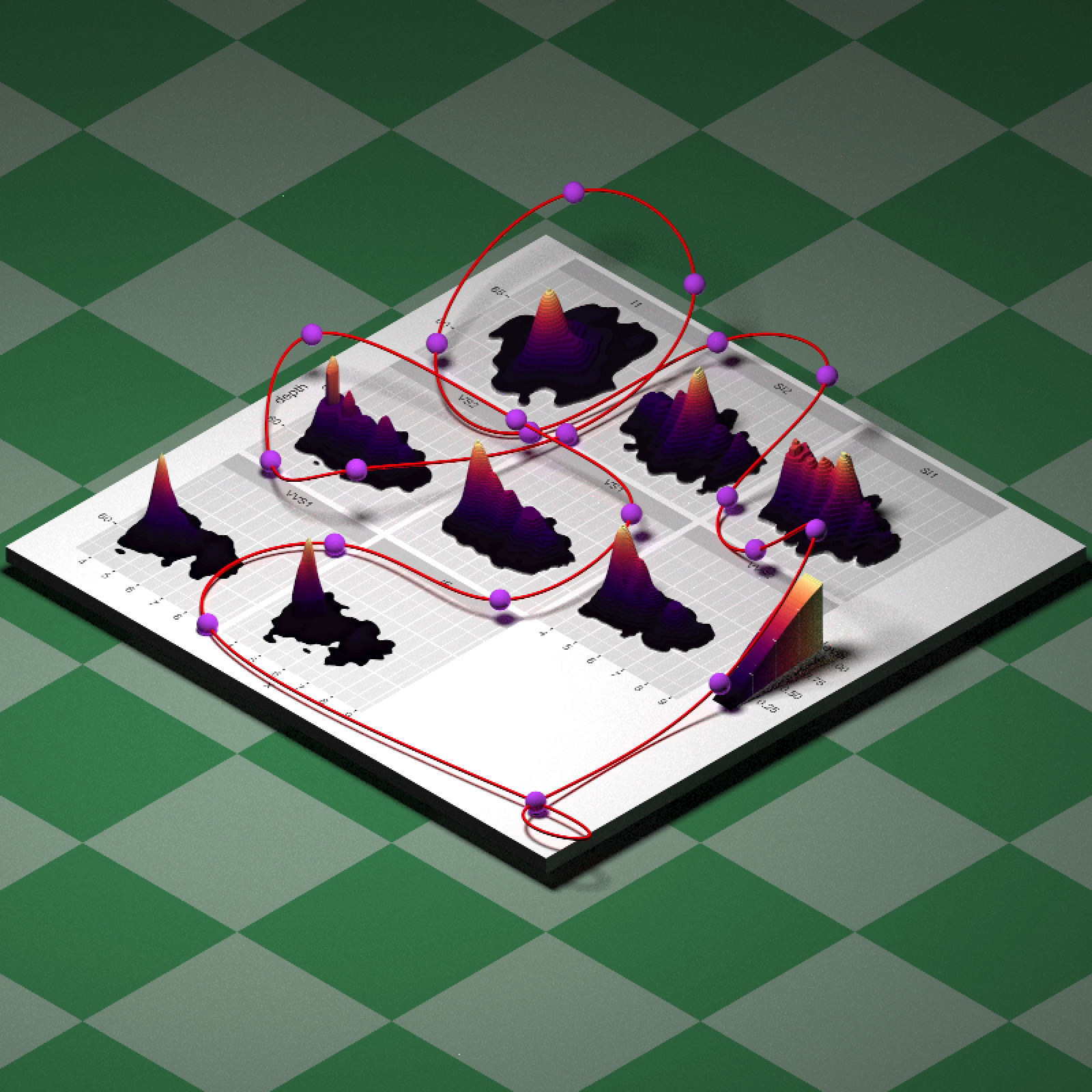
A real rollercoaster will have struts, and we can actually use the new animation function to generate these for us! Generating the camera motion is as simple as passing the above matrix of key frames to the generate_camera_motion() function. By default, the function places the camera at equally spaced intervals. Each row in the resulting data frame describes a camera position, orientation, and other properties. We can extract the camera position and use it to draw struts with cylinders.
camera_motion = generate_camera_motion(selected_points_new, closed=TRUE,
                                       frames = 360, constant_step = TRUE)
head(camera_motion)
## x y z dx dy dz aperture fov focal orthox orthoy upx
## 1 8.730352 0.3000000 9.121761 0 0 0 0 40 12.62995 1 1 0
## 4 8.724527 0.2680017 8.778475 0 0 0 0 40 12.37945 1 1 0
## 6 8.718827 0.2367145 8.435121 0 0 0 0 40 12.13364 1 1 0
## 8 8.713348 0.2066769 8.091653 0 0 0 0 40 11.89285 1 1 0
## 10 8.708196 0.1784969 7.748022 0 0 0 0 40 11.65746 1 1 0
## 13 8.703379 0.1522170 7.404231 0 0 0 0 40 11.42780 1 1 0
## upy upz
## 1 1 0
## 4 1 0
## 6 1 0
## 8 1 0
## 10 1 0
## 13 1 0strutlist = list()
for(i in 1:nrow(camera_motion)) {
strutlist[[i]] = segment(start = as.numeric(camera_motion[i,1:3])-c(0,0.05,0),
end =as.numeric(camera_motion[i,1:3])-c(0,20,0),
radius=0.02, material=diffuse(color="grey10"))
}
strutscene = do.call(rbind,strutlist)
disk(radius=1000,y=-1,
material=diffuse(checkerperiod = 6,checkercolor="#0d401b", color="#496651")) %>%
add_object(obj_model("ggplot.obj", y=-0.02, texture=TRUE, scale_obj = 1/100)) %>%
add_object(sphere(y=30,z=10,radius=5,material = light(intensity=40))) %>%
add_object(path(points=selected_points_new,width = 0.1, closed = TRUE,
material=diffuse(color = "red"))) %>%
add_object(keyscene_adj) %>%
add_object(strutscene) %>%
render_scene(lookfrom = c(20, 20, 20), fov = 0, ortho_dimensions = c(30, 30),
width = 800, height = 800, samples = 256)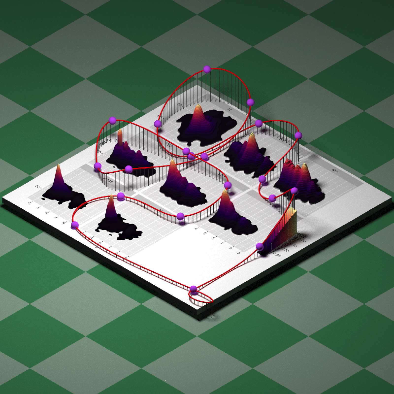
generate_camera_motion() do double duty and generate the coaster struts as well.
Now let’s generate our camera motion. By default, generate_camera_motion() looks at the origin—in order to look along our curve, we need to pass lookat positions as well as lookfrom. We actually want to look along the same path as our camera position, but just slightly in front of the current position. Rayrender provides a helper argument in generate_camera_motion() to do just that: set offset_lookat = 1 and the function will look ahead that distance on the Bézier curve. So we just need to pass two copies of selected_points_ne to the function. We can then pass this and our scene to render_animation() with debug = “preview” to quickly (in a few minutes) render a low-quality draft preview of the animation. I’ll also add an environment image to better orient us as we travel through the scene.
#Offset above track
selected_points_offset = selected_points_new
selected_points_offset[,2] = selected_points_offset[,2] + 0.15

camera_motion_real = generate_camera_motion(selected_points_offset, selected_points_offset,
                                            closed=TRUE, fovs = 90, constant_step = TRUE,
                                            frames=480,
                                            offset_lookat = 1)

disk(radius=1000,y=-1,
     material=diffuse(checkerperiod = 6,checkercolor="#0d401b", color="#496651")) %>%
  add_object(obj_model("ggplot.obj", y=-0.02, texture=TRUE, scale_obj = 1/100)) %>%
  add_object(path(points=selected_points_new,width=0.1, closed = TRUE,
                  material=diffuse(color="red"))) %>%
  add_object(strutscene) ->
  scene

render_animation(scene, camera_motion_real, environment_light = "quarry_03_4k.hdr",
                 debug="preview", filename="testroller", width=800,height=800)
Great! Except there’s a few spots where we’d end up with whiplash if we rode this in real life, as the viewpoint quickly changes direction at areas of high curvature. These quick transitions can be disorienting, so generate_camera_motion() includes an option to adjust for local curvature: setting curvature_adjust = “both” will adjust both the lookat and lookfrom positions so that the camera slows down in areas of high curvature, while maintaining the desired number of frames. Here’s a plot of each camera position showing the difference:
curvature_adjusted =  generate_camera_motion(selected_points_offset, selected_points_offset,
                                             closed=TRUE, fovs = 90, constant_step=FALSE,
                                             curvature_adjust = TRUE,curvature_scale = 60,
                                             frames=480,
                                             offset_lookat = 1)
curvature_adjusted$type = "Curvature Adjusted"
camera_motion_real$type = "Constant Step"
bothparts = rbind(camera_motion_real,curvature_adjusted)
ggplot(bothparts) +
  geom_point(aes(x=x,y=-z,color=y),alpha=0.7) +
  facet_wrap(~type) +
  coord_fixed() +
  scale_color_gradient("Height",low="#44ffff", high="purple") +
  theme(panel.background = element_rect(fill="grey20"),
panel.grid = element_line(color = "grey30")) 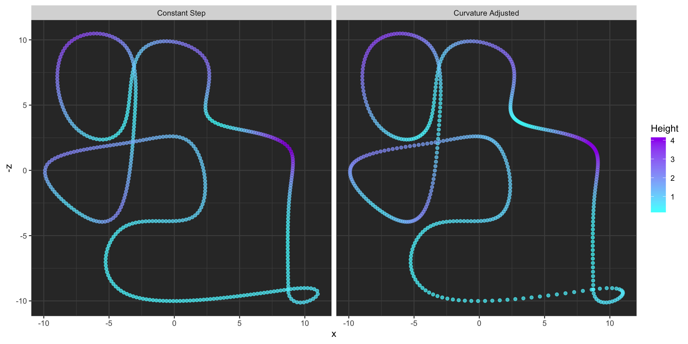
When we plot this version, we’ll see that the movement will slow down significantly when the underlying path changes quickly, which will prevent the nauseating quick movement we encountered before. The trade-off here is the path then moves more quickly through low curvature regions. Note that this option does not preserve key frame position and best works when the lookat and lookfrom positions are identical and you’re using using an offset, as otherwise the two paths can diverge.
Here’s a more extreme example using rayshader’s built-in montereybay dataset that includes a highly curved section. I’ve included the constant step version as well, so you can see how the two differ.
render_animation(…, debug=“preview”), which allows for quick low-quality renders of your final animation.
Another difference is the behavior of offset_lookat: when constant_step = TRUE, the function looks ahead a set distance along the curve. When constant_step = FALSE, however, the function uses the derivative of the Bézier curve to determine the offset position (I might change the behavior to be consistent across all versions later, but for now they behave slightly differently). Let’s generate an animation showing the difference. We’ll use the arrow primitive to show where the camera points at each interval (note the positions of the tip of the arrows). The animation interface currently only supports camera movement in a static scene, so we’ll have to animate this one the old fashioned way: generate each frame ourselves.
curvature_adjusted_arrow =  generate_camera_motion(selected_points_offset, selected_points_offset,
                                             closed=TRUE, fovs = 90, constant_step=FALSE,
                                             curvature_adjust = TRUE,
                                             frames=480,
                                             offset_lookat = 3)

curvature_constant_arrow =  generate_camera_motion(selected_points_offset, selected_points_offset,
                                             closed=TRUE, fovs = 90, constant_step=TRUE,
                                             frames=480,
                                             offset_lookat = 3)

lookatlist_adj = list()
lookatlist_con = list()

for(i in 1:nrow(curvature_constant_arrow)) {
  lookatlist_adj[[i]] = arrow(start = as.numeric(curvature_adjusted_arrow[i,1:3])+c(0,0.15,0),
                              tail_proportion = 0.7, radius_top = 0.4, radius_tail = 0.2,
                              end =as.numeric(curvature_adjusted_arrow[i,4:6]), material=glossy(color="#FFD700"))
  lookatlist_con[[i]] = arrow(start = as.numeric(curvature_constant_arrow[i,1:3])+c(0,0.15,0),
                              tail_proportion = 0.7, radius_top = 0.4, radius_tail = 0.2,
                              end =as.numeric(curvature_constant_arrow[i,4:6]), material=glossy(color="purple"))
}

for(i in 1:nrow(curvature_constant_arrow)) {
  disk(radius=1000,y=-1,
       material=diffuse(checkerperiod = 6,checkercolor="#0d401b", color="#496651")) %>%
    add_object(sphere(y=30,z=10,radius=5,material = light(intensity=80))) %>%
    add_object(path(points=selected_points_new,width=0.1, closed = TRUE,
                    material=diffuse(color="red"))) %>%
    add_object(lookatlist_adj[[i]]) %>%
    add_object(lookatlist_con[[i]]) %>%
    render_scene(lookfrom=c(20,20,20),fov=0,ortho_dimensions=c(22,22), width=800,height=800,
                    filename=sprintf("arrow_lookat_combined%i.png",i),clamp_value=10)
}offset_lookat = TRUE for constant_step = TRUE (which looks ahead on the curve) while the purple arrow represents the offset behavior with offset_lookat = TRUE (using local derivatives to determine the lookat position).
Now, let’s look at animating the lookat parameter separately. We’ll use the non-curvature adjusted path due to the aforementioned issues with the two paths diverging when curvature_adjust = TRUE. We’ll start with the lookat positions we already calculated, but now we’re going to change a couple parts: When we circle around the data, we’re going to change the focal point to look at the data (instead of straight ahead). This process is generally what you’d use when planning a 3D “tour” of your data: set a path for the camera to move along, and then direct the camera at points of interest as you move through the space. We’ll again use our clicking method to get the exact coordinates on the plot we want to focus on.
plot_image("raysurface.png")
vals2 = locator(n=2)
vals2$z = vals2$y
vals2$y = rep(2,length(vals2$y))
selected_focal_points = do.call(cbind,vals2)
selected_focal_point
## x y z
## [1,] 439.9366 2 1692.754
## [2,] 270.9225 2 1020.923#Center at origin, flip, and scale by 1/100 to match our rayrender model
selected_focal_points[,1] = (selected_focal_points[,1] - 2100/2)/100
selected_focal_points[,3] = -(selected_focal_points[,3] - 2100/2)/100The new focal points are plotted below in green.
disk(radius=1000,y=-1,
     material=diffuse(checkerperiod = 6,checkercolor="#0d401b", color="#496651")) %>%
  add_object(obj_model("ggplot.obj", y=-0.02, texture=TRUE, scale_obj = 1/100)) %>%
  add_object(sphere(y=30,z=-10,radius=5,material = light(intensity=40))) %>%
  add_object(path(points=selected_points,width=0.1, closed = TRUE, material=diffuse(color="red"))) %>%
  add_object(keyscene) %>%
  add_object(sphere(x=selected_focal_points[1,1],
                    y=selected_focal_points[1,2] + 3,
                    z=selected_focal_points[1,3],
                    radius=0.5, material=diffuse(color="green"))) %>%
  add_object(sphere(x=selected_focal_points[2,1],
                    y=selected_focal_points[2,2] + 3,
                    z=selected_focal_points[2,3],
                    radius=0.5, material=diffuse(color="green"))) %>%
  render_scene(lookfrom = c(0, 10, 0), fov = 0, ortho_dimensions = c(30, 30), camera_up = c(0,0,-1),
               width = 800, height = 800, samples = 256)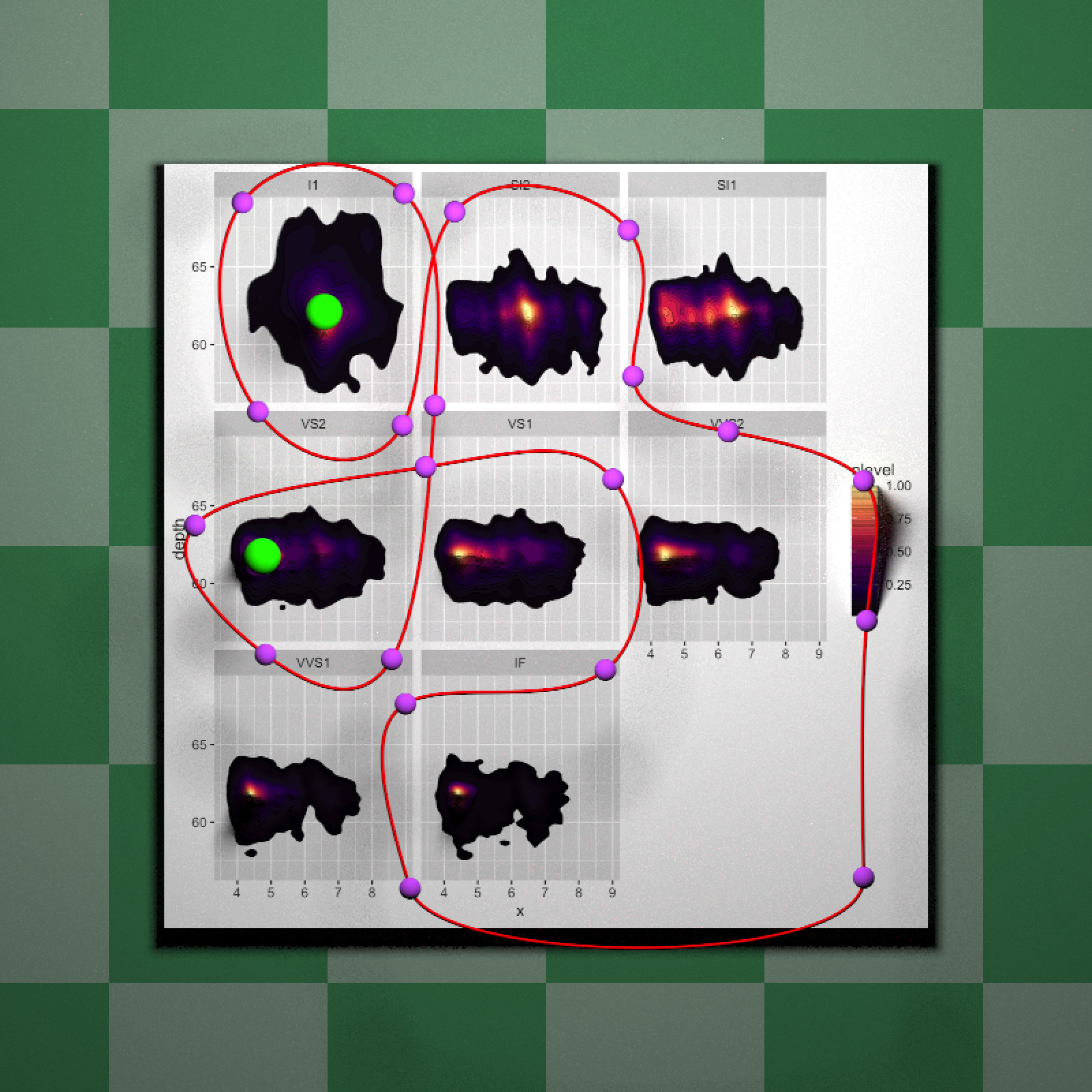
Let’s make the first peak the focal point from keyframes 8-11, and the second from keyframes 13-16. We’ll also have to manually offset the look position by playing around with matrix indices, since the offset argument doesn’t work when the point is stationary, as the derivative is undefined.
new_lookat_positions = selected_points_offset
new_lookat_positions[7:10,] = rbind(selected_focal_points[1,],selected_focal_points[1,],
                                    selected_focal_points[1,],selected_focal_points[1,])
new_lookat_positions[13:15,] = rbind(selected_focal_points[2,],selected_focal_points[2,],
                                     selected_focal_points[2,])

lookat_animated =  generate_camera_motion(selected_points_offset, new_lookat_positions,
                                          closed=TRUE, fovs = 90, constant_step = FALSE,
                                          curvature_adjust = "none",
                                          type = "bezier",
                                          frames=480,
                                          offset_lookat = 0)

#Offset by 5 steps along the path and recalculate the focal distance
lookat_animated2 = lookat_animated
lookat_animated2[,4:6] = rbind(lookat_animated[-(1:5),4:6],lookat_animated[(1:5),4:6])
lookat_animated2$focal = sqrt(apply(((lookat_animated2[,4:6]-lookat_animated2[,1:3])^2),1,sum))

render_animation(scene,lookat_animated2, width=1100,height=700,debug="preview",filename="animatelookat",
environment_light = "quarry_03_4k.hdr",)Cool! You now know how to create thrilling rides with your datasets in R. Use this power wisely (and don’t show Tufte).
And there’s your introduction to animation in R with rayrender! While animation is still a complex subject (and there are still pitfalls—Bézier curves can act pretty strangely at times!), rayrender now has a reasonably efficient and user-friendly method to create complex animations that don’t make you want to lose your lunch.
As a final note, this update also brings some pretty major improvements to rayrender’s underlying integrator: rayrender now has a high-quality Owen-scrambled Sobol sampler that converges far more quickly than any of the built-in samplers included thus far. This makes generating complex animations far less painful: rather than 500 samples per frame to get a clean image, now you might only need 1/4th of that amount! This is powered by the spacefillr package, a package that generates high-quality spacefilling sequences/sets that I submitted to the CRAN last month. Enjoy the time savings!