Dataviz Nanopost: Slices of the World
This is the first in a series of tiny posts where I show a data visualization along with the code used to generate it. I’ve always been annoyed at the lack of discoverability in Github Gists, so I’ve never really felt motivated to post code snippets there. Unlike github repos, gists tend to disappear into the void and never be seen again, unless linked by a blog post. And unlike Twitter, I can actually post the full code in a human (and text reader) friendly format. So I’m going to be posting my small “gists” here instead.
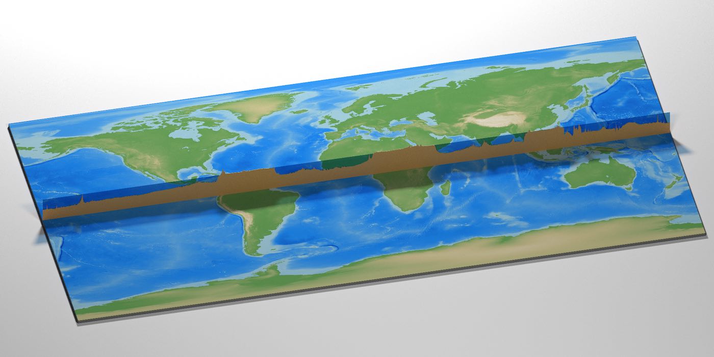
In this code snippet, I show how to use rayrender and rayshader to generate an animation of 3D slices of the earth’s bathymetry and topography. It’s basically a continuation of this blog post I released back in 2018, but now using the power of rayrender to make it prettier! Rendered in under 40 lines of code, too. Text/image overlay was applied post-processing using ffmpeg, which is the only step not included.
Here’s a link to the full-quality video if you’re interested (2000x1000).
Data source: NOAA (link)
Code:
library(rayshader)
library(rayrender)

#Generate world map from topographic/bathymetric data
matval = raster_to_matrix(raster::raster("ETOPO1_Ice_g_geotiff.tif"))
smallmat = resize_matrix(matval,0.25)
water_palette = colorRampPalette(c("darkblue", "dodgerblue", "lightblue"))(200)
bathysmall = height_shade(smallmat,range = c(min(smallmat),0), texture = water_palette)
smallmat %>%
  height_shade(range = c(0,max(smallmat))) %>%
  add_overlay(generate_altitude_overlay(bathysmall,smallmat,start_transition = 0)) %>%
  save_png("worldmap.png")

#Dimension of raster data is now 5400x2700
slices = c(seq(1,2700,by=3),2700)

for(i in 1:(length(slices)-1)) {
  smallmat[,slices[i]:slices[i+1]] -> temp

  #Generate 3D model
  temp %>%
    height_shade(range=range(smallmat)) %>%
    plot_3d(temp,zscale=50,water=TRUE,shadow=FALSE,soliddepth = -11000/50,
            watercolor="dodgerblue4",solidcolor = "#D2691E")
  save_obj("tempobj")
  rgl::rgl.clear()

  #Render image with rayrender
  xz_rect(xwidth=10000,zwidth=10000,y=-250) %>%
    add_object(xz_rect(xwidth=5400, zwidth=2700, y=-220,
                       material=diffuse(image_texture="worldmap.png"),angle=c(0,180,0))) %>%
    add_object(cube(xwidth=5400, zwidth=2700, ywidth = 200, y=-325,
                    material = diffuse(color="grey20"))) %>%
    add_object(sphere(radius=800,y=5000,z=-5000,material=light(intensity=70))) %>%
    add_object(sphere(radius=800,y=5000,z=5000,material=light(intensity=20))) %>%
    add_object(obj_model(z=mean(c(slices[i],slices[i+1]))-1350, "tempobj.obj",texture=TRUE)) %>%
    render_scene(lookfrom=c(-1000,3500,4500),fov=0,lookat=c(0,-220,0),
                 ortho_dimensions = c(6000,3000),samples=256,
                 filename=sprintf("slices%g.png",i),
                 width=2000,height=1000,clamp_value = 10, min_variance = 1e-5)
}