Loading and Visualizing OpenSky Network Flight Data in R (short)

Tl;dr: I will show you how to query the OpenSky REST API directly from R, load and clean the data, and then finally visualize it in 3D using the rayrender package—entirely in R. The OpenSky Network is a non-profit association that crowdsources flight path data. Volunteers set up sensors to read ADS-B messages sent out by aircraft, which contain the aircraft’s position and velocity. The volunteers then upload this data to the OpenSky network, which anyone can query via a REST API (although you need a free account for most of the functionality). I recently implemented a new path primitive in rayrender (to visualize smooth curves and lines in 3D) and needed some real-life data to test it on—this seemed like a pretty good source. Because I went through all the work to clean and visualize it myself, I figured I would make the process easier for others by showing what I did. Let’s get started!

First, let’s load the packages we’ll need. tidyverse loaded as a catch-all for data munging, httr is used to query the REST API, jsonlite for parsing the JSON data returned by the API, glue for some easy string manipulation, spData for the world map polygon, and rayrender to visualize it in 3D.

library(tidyverse) 
library(httr) 
library(jsonlite)
library(glue)
library(rayrender)
library(spData)

Here, you’ll need to put in your OpenSky username and password to access the API. You can sign up for a free account on opensky-network.org.

username = "xxxxxx"
password = "xxxxxx"

Since OpenSky is a EU-based non-profit, the coverage is much better in Europe. We are going to visualize all the departures on a single day from Frankfurt Airport (EDDF) in Germany. This involves interacting with two services in the OpenSky REST API: one that gives us the departures from a specific airport, and one that will give us the flight tracks for those specific flights. We can only read up to 2 hours at a time for the departure API, so we will loop through every hour and collect the departing flights into a list. Then, we’ll pass those flights into the second endpoint to get the actual tracks.

We are going to be using the httr package to interact with the API. It’s pretty straightforward: a key-value pair is specified in a list to the query argument in httr::GET. We’ll pass the airport and the timespan (here, in Unix time) to get a list of departures. After that’s done, we’ll then loop through all those departures to extract the track information, growing a list of our results.

tracklist = list()
counter_tracks = 1

#This is the string we'll use to access the departures API
path = glue("https://{username}:{password}@opensky-network.org/api/flights/departure?")

#This is the string we'll use to access the tracks API
trackpath = glue("https://{username}:{password}@opensky-network.org/api/tracks/all?")

for(j in 1:23) {
  begintime = as.numeric(as.POSIXct(sprintf("2020-08-10 %0.2d:01:00 EST",j-1)))
  endtime = as.numeric(as.POSIXct(sprintf("2020-08-10 %0.2d:01:00 EST",j)))
  
  #Get the flights departing within that hour
  request = GET(url = path, 
                query = list(
                   airport = "EDDF",
                   begin = begintime,
                   end = endtime))
  response = content(request, as = "text", encoding = "UTF-8")
  df = data.frame(fromJSON(response, flatten = TRUE))

  #Read the actual tracks
  for(i in 1:nrow(df)) {
    request_track = GET(url = trackpath, 
                        query = list(
                          icao24 = df$icao24[i],
                          time = begintime+1800)) #Offset to the middle of the hour
    
    response_track = content(request_track, as = "text", encoding = "UTF-8")
    if(response_track != "") {
      tracklist[[counter_tracks]] = data.frame(fromJSON(response_track, flatten = TRUE))
    }
    counter_tracks = counter_tracks + 1
  }
}

This should take a few minutes to run, but will give us our flight path trajectory data. Some entries will contain only a single row telling us there were no departing flights: let’s filter those out by pulling out only data.frames with more than one row.

newtracklist = list()
for(i in 1:length(tracklist)) {
  if(!is.null(tracklist[[i]])) {
    if(nrow(tracklist[[i]]) > 1) {
      newtracklist[[i]] = tracklist[[i]]
    }
  }
}

Now, let’s combine all those tracks into a single data.frame and extract the ICAO24 codes for each aircraft. Each ICAO24 code is unique to each aircraft and thus is a good way to track a specific aircraft in the sky.

fulltracks = do.call(rbind,newtracklist)
unique_codes = unique(fulltracks$icao24)

For fun, let’s load the world polygon data from the spData package and plot our tracks with ggplot2 (just so we have an idea of what the data looks like):

worldmap = spData::world

ggplot() + 
  geom_sf(data=worldmap) +
  geom_path(data=fulltracks, aes(x=path.3,y=path.2, color=icao24)) + 
  theme(legend.position = "none")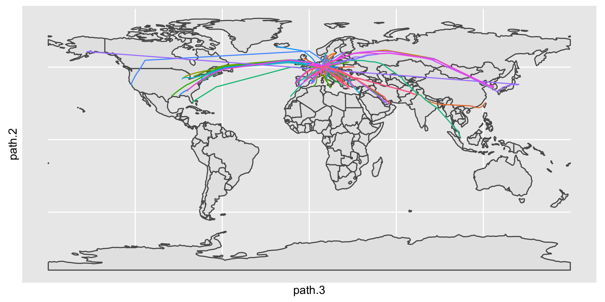

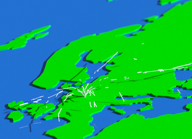
Figure 1: Quick preview.

Cool! Now let’s render our flight track data in 3D using rayrender. We’ll turn the world polygon into an extruded 3D surface, add a glossy blue rectangle to represent the ocean, and then generate our path() objects and pass them into the scene. By setting u_min and u_max in the the path() function, we can draw only a portion of the full aircraft trajectory and animate it over time.

worldpoly = extruded_polygon(worldmap,material=diffuse(color="darkgreen"))
len_u_min = seq(0,1,length.out = 361)[-1]
len_u_max = len_u_min + 0.03
len_u_max[len_u_max > 1] = 1

for(j in 1:360) {
  path_mat_list = list()
  for(i in 1:length(unique_codes)) {
    path_mat_list[[i]] = filter(fulltracks, icao24 == unique_codes[i]) %>% 
      select(path.2,path.3,path.4) %>% 
      mutate(z=path.2, y=path.4/5000, x=-path.3) %>% #Scale the altitude and flip the x-axis
      select(x,y,z)  %>% 
      as.matrix() %>% 
      path(material = diffuse(color="white"), width=0.025, type="cylinder", 
           u_max = len_u_max[j], u_min = len_u_min[j])
  }
    
  #Combine all the path objects into a single scene
  all_tracks_ray = dplyr::bind_rows(path_mat_list)
  
  xz_rect(y=0.7,xwidth=1000,zwidth=1000,material=glossy(color="#00144a")) %>% 
    add_object(worldpoly) %>% 
    add_object(group_objects(all_tracks_ray, group_translate = c(0,1,0))) %>%  
    render_scene(lookfrom=c(1000,700,-1000),lookat=c(-12,0,50.1),fov=1.4,
                 samples=64,sample_method = "stratified",
                 environment_light = "autumn_park_1k.hdr", #HDR image from hdrihaven.com
                 width = 1200, height=1200, aperture=20,
                 filename=glue::glue("flight_anim{j}"))
}

We can then combine all these images into a movie using the av package:

av::av_encode_video(glue::glue("flight_anim{1:360}.png"), output = "flight_anim.mp4", framerate = 30)

Figure 2: Video from image frames.

Hope you liked this mini-tutorial! Follow me on Twitter and sign up for my listserv if you want to read more content like this.