Pathtracing Neon Landscapes in R
I’ve been having fun the last few months adhering to a relatively rapid open-source development schedule (as much as you can call a one-man project driven by a Mac Stickies window a “schedule”) with constant releases of rayrender, rayshader, and now rayimage. And in that time, I’ve managed to push lots of cool features, like true pathtracing of terrain in rayshader and realistic layered dielectrics in rayrender. And, as the author of the packages, it’s easy for me to sit down and immediately start creating with them. But there’s one downside of that singular focus on development: a complete lack of tutorials for other people on how to use the software. And, as the point of a package is to share code with other people, this is a problem.
Don’t get me wrong—I make sure to update the documentation and add examples to the package, and I have pkgdown websites that turn those examples into easily referenceable HTML. But documentation examples are bound by simplicity: you need remove all the delightful complexity of real world examples so you can show off the building blocks of the API. Not great for flexing to show off what your package can do. So this is the first in a series of blog posts where I do just that: show (with all the code) how to use these packages to craft something awesome!
So let’s get started! One feature I added to rayrender last year was a new object: line segments. Line segments are thick 3D cylinders, specified with a start point, end point, and radius. That parameterization is super-useful, as lots of data are specified in terms of line segments: e.g. polygon edges, time series, contours lines. Contour lines in particular are well-suited for a 3D representation, because they’re actually representing 3D data: lines of constant elevation on an underlying 3D surface. So when I saw this tweet, I saw an opportunity to use them:
@tylermorganwall Question for you! Do you think it would be possible to modify rayshader to do something in the style of @mjmurdoc’s art? pic.twitter.com/u2Qj43TBLT
— Jacqueline Nolis (@skyetetra) February 5, 2020
Let’s recreate a neon wireframe scene similar to this, but entirely in R! Not with rayshader though (it’s meant to work with raster data), but with rayrender. We’ll need a couple things to make this work:
- An underlying landscape to transform into retro VR neon lines.
- Code to generate line segments representing the contour lines for said surface.
- Software to construct the 3D scene and render it.
We’ll use the built-in R dataset volcano for the landscape, Claus Wilke’s isoband package to generate the contours, and rayrender to build the scene and render it entirely in R.
First, let’s start by building the contour lines. We’ll first start by plotting the 3D map with rayshader and creating a 3D video, so you know what the surface looks like:
library(rayshader)
volcano %>%
  sphere_shade() %>%
  add_shadow(ray_shade(volcano,zscale=3),0.3) %>%
  plot_3d(volcano, zscale=3, fov=30)
render_movie("basic_video.mp4", title_text = "Basic rayshader plot",
             title_bar_color = "red", title_bar_alpha = 0.3)
rgl::rgl.close()
Let’s create a contour plot of this data, using isoband::isolines(). We’ll then plot the data using ggplot2 + sf.
library(ggplot2)

volcano_contours = isoband::isolines(x = 1:ncol(volcano),
                                     y = 1:nrow(volcano),
                                     z = volcano,
                                     levels=seq(120,190,by=10))

contours = isoband::iso_to_sfg(volcano_contours)
sf_contours = sf::st_sf(level = names(contours), geometry = sf::st_sfc(contours))

ggplot(sf_contours) + geom_sf(aes(color = level))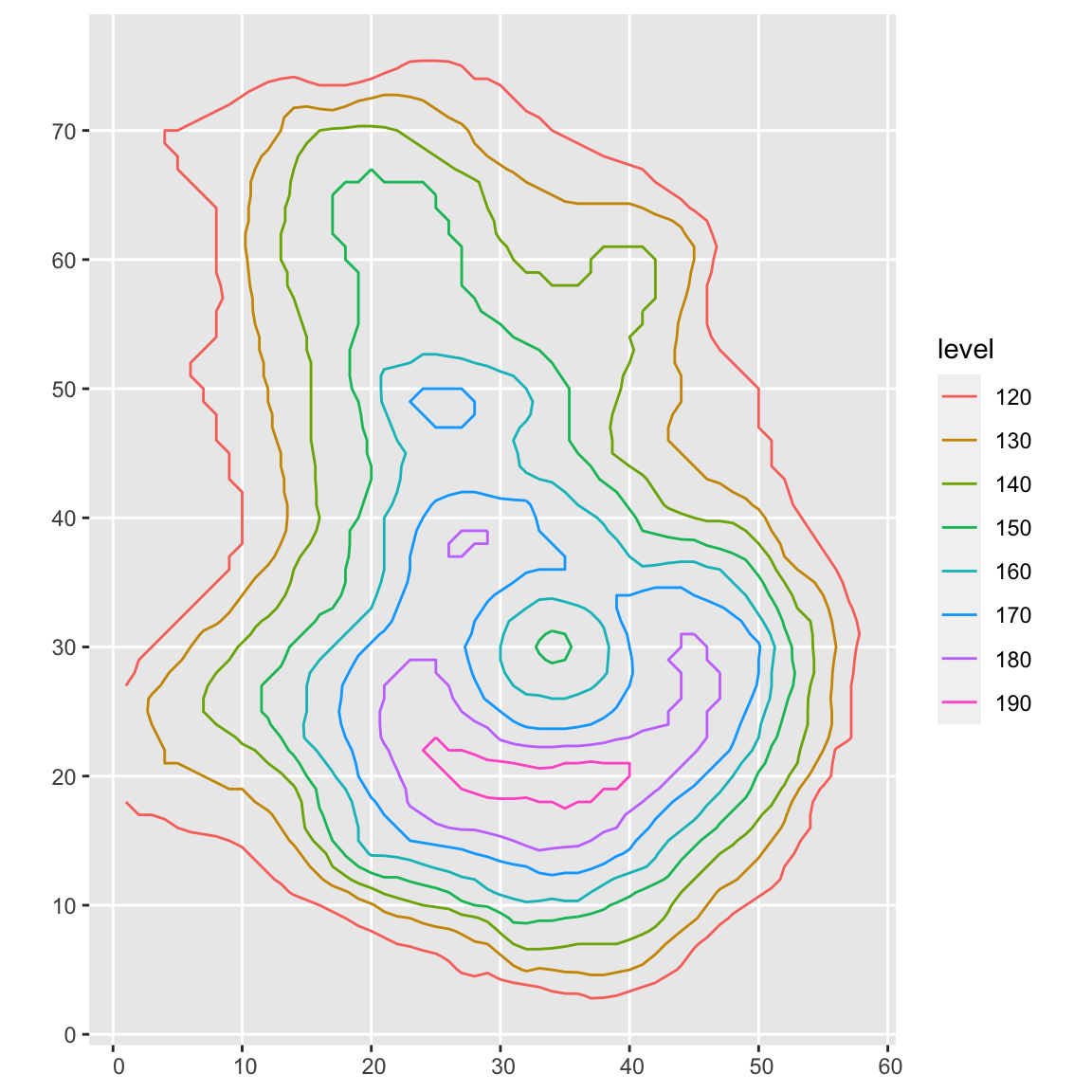
Cool! Let’s pull each line out of the original volcano_contour object. Each contour level consists of x and y coordinates labeling the path , and an ID coordinate that separates different paths on the same altitude (the path doesn’t have to be continuous–the ID specifies each contiguous “chunk” at a certain level). The name of the level is the altitude.
We’ll loop through each altitude layer, extract the x and y-coordinates for the path of the lines, and then add the resulting line segments to a list collecting all the elements of the scene. The volcano dataset starts at 94m, so we’ll subtract off some elevation to get it closer to the ground, compress it by a factor of 5 so it fits in our screen, and add an x/z offset to center the model. Since each element is a row in a data.frame, we’ll bind all the rows together in the list to get the resulting scene to pass to rayrender.
library(rayrender)

scenelist = list()
counter = 1

for(i in 1:length(volcano_contours)) {
  heightval = as.numeric(names(volcano_contours)[i])
  uniquevals = table(volcano_contours[[i]]$id)
  for(k in 1:length(uniquevals)) {
    tempvals = volcano_contours[[i]]
    tempvals$x = tempvals$x[tempvals$id == k]
    tempvals$y = tempvals$y[tempvals$id == k]
    for(j in 1:(length(tempvals$x)-1)) {
      scenelist[[counter]] = segment(start = c(tempvals$x[j]-30,
                                               (heightval-80)/5-3,
                                               tempvals$y[j]-44),
                                     end   = c(tempvals$x[j+1]-30,
                                               (heightval-80)/5-3,
                                               tempvals$y[j+1]-44),
                                     radius = 0.3,
                                     material = diffuse(color=heat.colors(9)[i]))
      counter = counter + 1
    }
  }
}

fullscene = do.call(rbind, scenelist)

generate_ground(material = diffuse(color="grey20")) %>%
  add_object(fullscene) %>%
  render_scene(lookfrom = c(0,80,150), lookat = c(0,-1,-10), samples = 200,
               aperture = 0, fov = 25, width = 800, height = 800)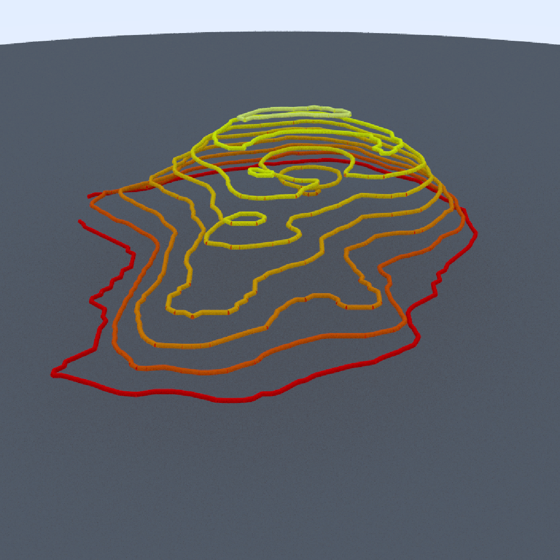
Since the lines don’t have end caps, we can see small breaks between each segment in a layer. We will add spheres with the same radius as our lines at each start point to cover up these breaks. We’ll also change the surface to a dark metallic rough mirror (roughness specified by the non-zero fuzz argument in metal()), and change the line material to a glowing light with the light() material. Adding a light will also automatically turn off the ambient lighting in the scene, so the only light source will be the glowing contour lines.
scenelist = list()
counter = 1

for(i in 1:length(volcano_contours)) {
  heightval = as.numeric(names(volcano_contours)[i])
  uniquevals = table(volcano_contours[[i]]$id)
  for(k in 1:length(uniquevals)) {
    tempvals = volcano_contours[[i]]
    tempvals$x = tempvals$x[tempvals$id == k]
    tempvals$y = tempvals$y[tempvals$id == k]
    for(j in 1:(length(tempvals$x)-1)) {
      scenelist[[counter]] = segment(start = c(tempvals$x[j]-30,
                                               (heightval-80)/5-3,
                                               tempvals$y[j]-44),
                                     end   = c(tempvals$x[j+1]-30,
                                               (heightval-80)/5-3,
                                               tempvals$y[j+1]-44),
                                     radius = 0.3,
                                     material = light(intensity = 3,
                                                      color=heat.colors(9)[i]))
      counter = counter + 1

      #Add a sphere at each corner
      scenelist[[counter]] = sphere(x = tempvals$x[j]-30,
                                    y = (heightval-80)/5-3,
                                    z = tempvals$y[j]-44,
                                    radius = 0.3,
                                    material = light(intensity = 3,
                                                     color=heat.colors(9)[i]))
      counter = counter + 1
    }
  }
}

fullscene2 = do.call(rbind, scenelist)

generate_ground(material = metal(color="grey20", fuzz=0.05)) %>%
  add_object(fullscene2) %>%
  render_scene(lookfrom = c(0,80,150), lookat = c(0,-1,-10), samples = 200,
               aperture = 0, fov=25, tonemap = "reinhold",
               width = 800, height = 800)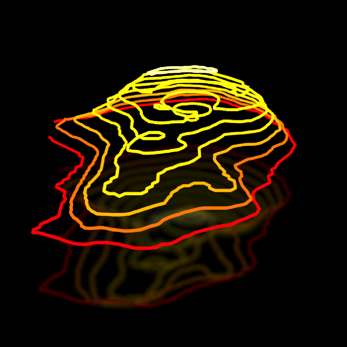
The only problem is the lines, while lit, aren’t glowing like neon. A very slight bloom effect is added by default in render_scene() to anti-alias lights (which is difficult to do in pathtracing, especially when tone mapping), but we can ramp up that effect to get a intense glowing aura surrounding our lines. Let’s set bloom = 5 in render_scene() to improve this effect.
generate_ground(material = metal(color="grey20", fuzz=0.05)) %>%
  add_object(fullscene2) %>%
  render_scene(lookfrom = c(0,80,150), lookat=c(0,-1,-10), samples = 200,
               aperture = 0, fov = 25, bloom = 5, tonemap = "reinhold",
               width = 800, height = 800)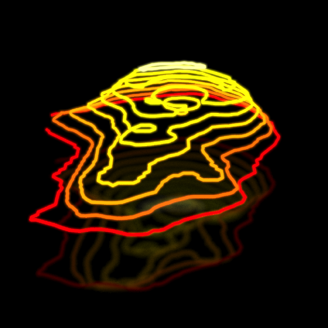
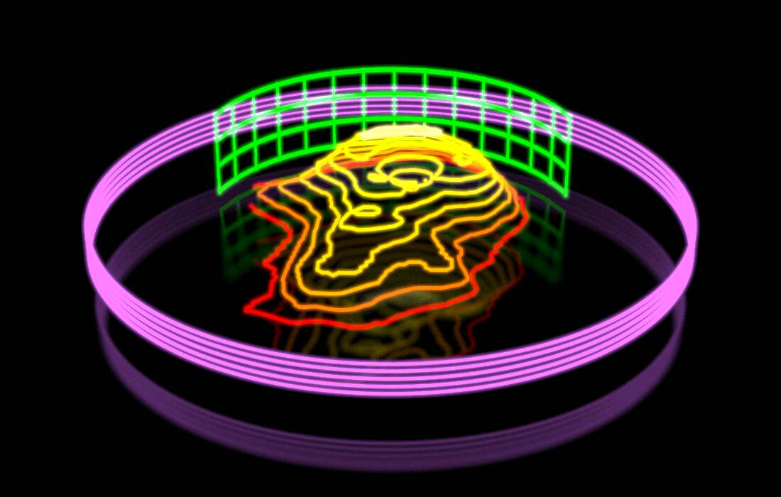
Nice. Now, in the style of the original image by @mjmurdoc, let’s add a green circular grid in the background. We’ll first start by generating the vertical bars in 10 degree increments subtending an arc of a circle, and then add the circular horizontal stripes by rendering a truncated cylinder in the same arc. We’ll have to render the cylinder twice, slightly offset and normals flipped, because light in rayrender is only emitted from the “outward” face of objects, and we’re going to see both sides when we orbit around the scene. I’m also going to add a glowing purple circle below everything (by adding a flat disk with a large inner radius).
green_light = light(color="green", intensity = 3)

grid = list()
counter = 1
for(i in seq(110,250,by=10)) {
  grid[[counter]] = segment(start=c(sinpi(i/180)*40,
                                    -0.5,
                                    cospi(i/180)*40-20),
                            end = c(sinpi(i/180)*40,
                                    18.5,
                                    cospi(i/180)*40-20),
                            radius=0.25,
                            material = green_light)
  counter = counter + 1
}

green_grid_vertical = do.call(rbind, grid)

generate_ground(material = metal(color="grey20",fuzz=0.05)) %>%
  add_object(green_grid_vertical) %>%
  add_object(fullscene2) %>%
  render_scene(lookfrom = c(0,80,150),lookat = c(0,-1,-10), samples = 40,
               aperture = 0, fov = 25, bloom = 5, tonemap="reinhold",
               width=800,height=800)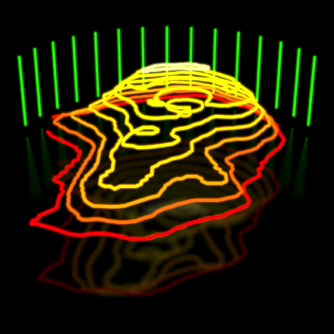
#Generate the horizontal grid stripes
cylinder(radius=40, z=-20,material = green_light,
         phi_min = 200, phi_max = 340, flipped = FALSE) %>%
  add_object(cylinder(radius=40, y=6,z=-20,material = green_light,
                      phi_min = 200, phi_max = 340, flipped = FALSE)) %>%
  add_object(cylinder(radius=40, y=12,z=-20,material = green_light,
                      phi_min = 200, phi_max = 340, flipped = FALSE)) %>%
  add_object(cylinder(radius=40, y=18,z=-20,material = green_light,
                      phi_min = 200, phi_max = 340, flipped = FALSE)) %>%
  add_object(cylinder(radius=40, z=-20.01,material = green_light,
                      phi_min = 200, phi_max = 340)) %>%
  add_object(cylinder(radius=40, y=6,z=-20.01,material = green_light,
                      phi_min = 200, phi_max = 340)) %>%
  add_object(cylinder(radius=40, y=12,z=-20.01,material = green_light,
                      phi_min = 200, phi_max = 340)) %>%
  add_object(cylinder(radius=40, y=18,z=-20.01,material = green_light,
                      phi_min = 200, phi_max = 340)) ->
green_grid_horizontal

#Purple base disk
base_disk = disk(inner_radius = 60, radius=61, z=-10,
                 material = light(intensity = 3, color="purple")) %>%
  add_object(disk(inner_radius = 60, radius=61, y=-0.1, z=-10,
                  material = light(intensity = 3, color="purple"), flipped=TRUE))

generate_ground(material = metal(color="grey20",fuzz=0.05)) %>%
  add_object(green_grid_vertical) %>%
  add_object(green_grid_horizontal) %>%
  add_object(base_disk) %>%
  add_object(fullscene2) %>%
  render_scene(lookfrom = c(0,80,150), lookat=c(0,-1,-10), samples = 200,
               aperture = 0, fov = 25, bloom = 5, tonemap = "reinhold",
               width = 800, height = 800)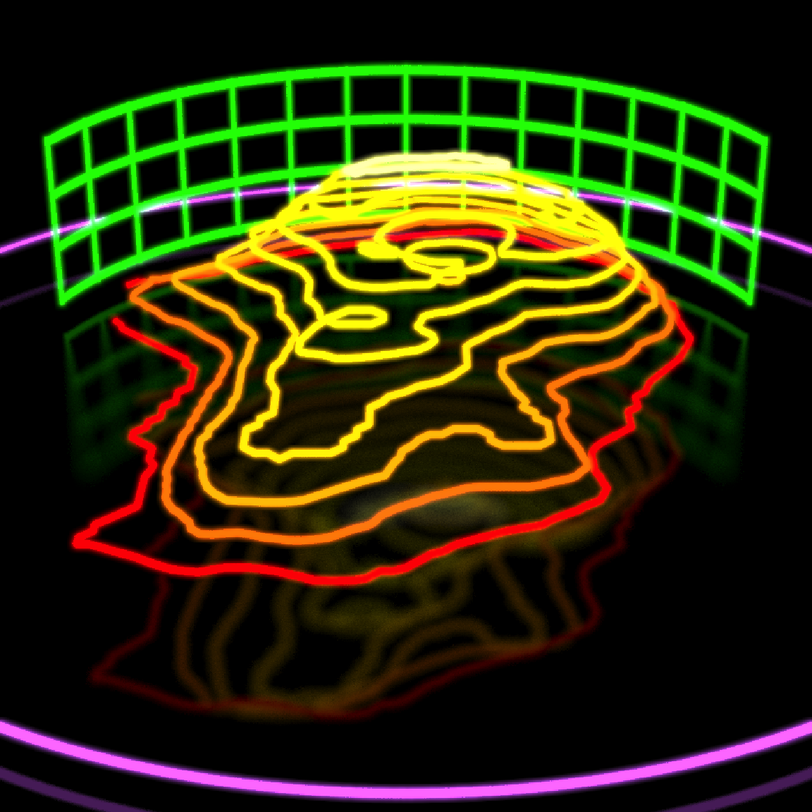
Now let’s orbit around the scene! We’ll rotate the camera lookfrom position in a circle around the volcano and save each image to a frame, and then combine them all into a video. We’ll also double the distance and change the field of view (fov) slightly, so the entire scene stays in frame as we circle around it. And let’s duplicate and animate the base disk in a sine wave with slight offsets, for a fun effect (and to show off the group_objects() function in rayrender).
xpos = 300 * sinpi(1:360/180)
zpos = 300 * cospi(1:360/180)

disk_height  = 6+6*sinpi(1:360/180*2)
disk_height2 = 6+6*sinpi(1:360/180*2+15/180)
disk_height3 = 6+6*sinpi(1:360/180*2-15/180)
disk_height4 = 6+6*sinpi(1:360/180*2+30/180)
disk_height5 = 6+6*sinpi(1:360/180*2-30/180)


for(i in seq(1,360,by=1)) {
  generate_ground(material = metal(color="grey20",fuzz=0.05)) %>%
    add_object(green_grid_vertical) %>%
    add_object(green_grid_horizontal) %>%
    add_object(group_objects(base_disk, group_translate = c(0,disk_height[i],0))) %>%
    add_object(group_objects(base_disk, group_translate = c(0,disk_height2[i],0))) %>%
    add_object(group_objects(base_disk, group_translate = c(0,disk_height3[i],0))) %>%
    add_object(group_objects(base_disk, group_translate = c(0,disk_height4[i],0))) %>%
    add_object(group_objects(base_disk, group_translate = c(0,disk_height5[i],0))) %>%
    add_object(fullscene2) %>%
    render_scene(lookfrom = c(xpos[i],160,zpos[i]-10),lookat = c(0,-1,-10), samples = 200,
                 aperture = 0, fov = 22, bloom = 5, tonemap = "reinhold",
                 width = 800, height = 800, filename = sprintf("neonvolcano%d",i))
}


av::av_encode_video(sprintf("neonvolcano%d.png",seq(1,360,by=1)), framerate = 30,
                    output = "neonvolcano.mp4")
We can also include depth of field to create a “miniature holographic volcano” effect by increasing the aperture setting in render_scene(). This makes only a certain slice of the scene in focus, and as we move away from that distance objects will become progressively more blurry. Depth of field is only of those effects that’s difficult to implement well in a rasterizing 3D renderer, but fairly straightforward in a pathtracer.
for(i in seq(1,360,by=1)) {
  generate_ground(material = metal(color="grey20",fuzz=0.05)) %>%
    add_object(green_grid_vertical) %>%
    add_object(green_grid_horizontal) %>%
    add_object(group_objects(base_disk, group_translate = c(0,disk_height[i],0))) %>%
    add_object(group_objects(base_disk, group_translate = c(0,disk_height2[i],0))) %>%
    add_object(group_objects(base_disk, group_translate = c(0,disk_height3[i],0))) %>%
    add_object(group_objects(base_disk, group_translate = c(0,disk_height4[i],0))) %>%
    add_object(group_objects(base_disk, group_translate = c(0,disk_height5[i],0))) %>%
    add_object(fullscene2) %>%
    render_scene(lookfrom = c(xpos[i],160,zpos[i]-10), lookat = c(0,-1,-10), samples =200,
                 aperture = 30, fov=22, bloom = 5, tonemap="reinhold",
                 width = 800, height = 800, filename=sprintf("neonvolcanomini%d",i))
}

av::av_encode_video(sprintf("neonvolcanomini%d.png",seq(1,360,by=1)), framerate = 30,
                    output = "neonmini.mp4")
The original image that inspired this also had a slight reddish tint, so we’ll use the rayimage package to add a semi-transparent red overlay to all the images to achieve the same effect. rayimage is a new package in R that allows you to manipulate images in R as arrays, adding titles/image overlays, changing image orientation, and performing image convolutions (like our bloom effect).
library(rayimage)

red_overlay = array(1,dim=c(3,3,3))
red_overlay[,,1] = 0.7
red_overlay[,,2] = 0
red_overlay[,,3] = 0

for(i in seq(1,360,by=1)) {
  add_image_overlay(sprintf("neonvolcano%d.png",i), red_overlay, alpha = 0.25, preview=TRUE,
                    filename = sprintf("neonvolcanored%d.png",i))
}
av::av_encode_video(sprintf("neonvolcanored%d.png",seq(1,360,by=1)), framerate = 30,
                    output = "neonminired.mp4")
And that’s it! I hope you enjoyed this little mini-tour on creating and animating a 3D scene entirely in R, and has given you some inspiration for making slick 3D scenes of your own. If you do generate a scene you want to show off, share it on Twitter with the hashtag’s #rstats and #rayrender! There’s a great community of people who would love to see what you came up with.