Plinko Statistics: Insights from the Bean Machine
A Galton board (aka a “Bean Machine”) is an interesting mix of chaos and predictability: a single ball’s path is unpredictable, yet the behavior of a mass of balls results in a remarkably consistent result. It’s a toy that cuts right to the core of statistics: one measurement doesn’t tell you much about a system, but many measurements in aggregate do. Combining those concepts with all fun of plinko/pachinko/peggle and you have an excellent little system that can illustrate a great number of statistical concepts. It’s no surprise that it makes an early appearance in most statistics curriculum. However, most instructors only use it as an illustration of the Central Limit Theorem: a series of binary choices results in a normal distribution. This is a shame, since you can illustrate so much more if you look a little deeper–and that’s what this blog post is going to do.
I was inspired to make this post after @coolbutuseless released the chipmunkcore/chipmunkbasic package: an R wrapper around the Chipmunk2D physics library. Wrapping a physics library in R had long been on my “maybe one day” todo list, so I was glad someone beat me to the punch–less work for me! The package allows you to build a fixed scene out of rectangles and then place movable objects (circles, spheres, and polygons) that can interact with each other, the scene, and a gravitational force.
With the package, @coolbutuseless released a slick demo (with code) animating a Galton board with ggplot2. Awesome–but what if we could render a 3D visualization of the same data that gives us something more true-to-life? Still a 2D simulation, but rendered like the real thing. If only there was a package that could render complex 3D scenes directly in R… which of course there is! We will be using the rayrender package to generate our 3D renders. I wrote rayrender to create high quality 3D visualizations in R, without having to export your data to another program. Rayrender allows you to easily craft 3D scenes out of a wide range of primitive objects. It renders scenes using pathtracing to produce a photorealistic result.
Let’s jump right into writing code. First we’ll load the required packages. You have to install the Chipmunk2D library on your computer: easy on macOS if you use homebrew brew install chipmunk and a bit more involved on Ubuntu. You can see additional instructions I provided on the Github repo README, expand the “Click to show instructions for ubuntu - method 1” tab). Once that’s done, install {chipmunkcore} and {chipmunkbasic} from Github). On Windows–sorry, I have no idea!
emotes::install_github("coolbutuseless/chipmunkcore")
remotes::install_github("coolbutuseless/chipmunkbasic")
library(chipmunkcore)
library(chipmunkbasic)
library(rayrender)
We’ll then copy some of the code @coolbutuseless used to generate the Galton board and extract a rayrender scene. A Galton board consists of three areas: The funnel that ensures the balls fall from approximately the same point:
# Add funnel segments
generate_funnel_scene = function(color="red") {
  xz_rect(x=-67/2-3,y=125,xwidth=83.60024,angle=c(0,0,36.73283),zwidth=5,
                   material=diffuse(color=color)) %>%
    add_object(xz_rect(x=67/2+3,y=125,xwidth=83.60024,angle=c(0,0,-36.73283),zwidth=5,
                     material=diffuse(color=color))) %>%
    add_object(yz_rect(x=-3,y=95, ywidth=10,zwidth=5, material=diffuse(color=color))) %>%
    add_object(yz_rect(x=3,y=95, ywidth=10, zwidth=5,material=diffuse(color=color)))
}

funnelscene = generate_funnel_scene()

generate_studio(width = 1000, height = 1000,depth=-5) %>%
    add_object(funnelscene) %>%
    add_object(sphere(y=200,z=100,radius=20,material=light(intensity = 40))) %>%
    render_scene(lookfrom=c(0,150,100),fov=90,lookat=c(0,50,0),samples=512,
                 clamp_value = 10, sample_method = "stratified", width=800,height=800)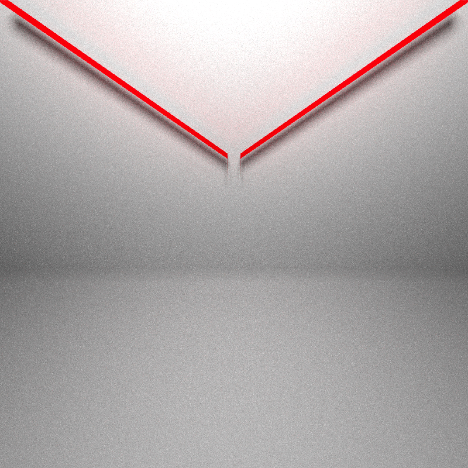
Next comes the pegs that interrupt the flow of the balls. These force the balls left or right. They are actually small rectangles in the simulation, but here we’ll represent them with cylinders (they are small enough that you can’t visually tell the difference):
#Generate pegs
generate_peg_scene = function(pegs = 15, color="red") {
  cm = Chipmunk$new(time_step = 0.005)
  for (i in 1:pegs) {
    y = 90 - i * 3
    if (i %% 2 == 1) {
      xs = seq(0, 40, 2)
    } else {
      xs = seq(1, 40, 2)
    }
    xs = 1.0 * sort(unique(c(xs, -xs)))

    w = 0.05
    xstart = xs - w
    xend   = xs + w

    for (xi in seq_along(xs)) {
      cm$add_static_segment(xstart[xi], y+0.01,  xend[xi],  y-0.01)
    }
  }

  #Convert chipmunk pegs into a rayrender scene:
  cm$get_static_segments() -> peg_seg
  peglist = list()
  for(i in 1:nrow(peg_seg)) {
    peglist[[i]] = cylinder(x=peg_seg$x1[i]+0.05, y=peg_seg$y1[i],
                            angle=c(90,0,0),radius=0.1, length=5,material=diffuse(color=color))
  }
  do.call(rbind,peglist)
}

pegscene = generate_peg_scene()

generate_studio(width = 1000, height = 1000,depth=-5) %>%
    add_object(funnelscene) %>%
    add_object(pegscene) %>%
    add_object(sphere(y=200,z=100,radius=20,material=light(intensity = 40))) %>%
    render_scene(lookfrom=c(0,130,100),fov=50,lookat=c(0,60,0),samples=512,
                 clamp_value = 10, sample_method = "stratified", width=800,height=800)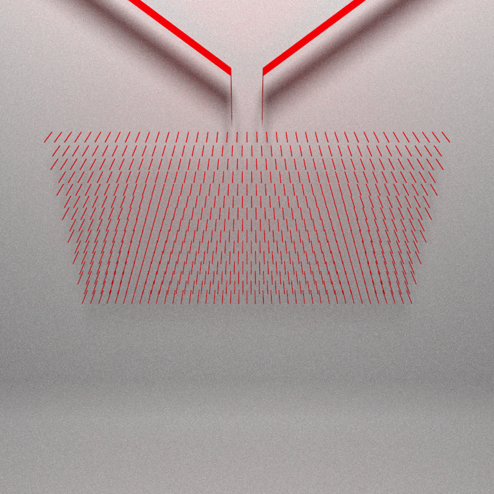
And finally the buckets that hold the balls:
generate_slot_scene = function(pegs=15, color="red") {
  cm = Chipmunk$new(time_step = 0.005)
  floor = 85 - pegs*3 - 40
  width = 50
  for (x in seq(-width, width, 5)) {
    cm$add_static_segment(x, floor,  x,  85 - pegs*3)
  }

  cm$get_static_segments() -> slots

  slotlist = list()
  counter = 1
  for(i in 1:nrow(slots)) {
    slotlist[[counter]] = cube(x=slots$x1[i],y=85 - pegs*3-20, xwidth=0.05,
                               ywidth=40,zwidth=5,material=diffuse(color=color))
    counter = counter + 1
  }
  #Bottom of the bucket:
  slotlist[[counter]] = cube(y=floor, xwidth=100,zwidth=5,ywidth=0.05, material=diffuse(color=color))
  slotscene = do.call(rbind,slotlist)
  slotscene
}

slotscene = generate_slot_scene()

generate_studio(width = 1000, height = 1000,depth=-5) %>%
  add_object(funnelscene) %>%
  add_object(pegscene) %>%
  add_object(slotscene) %>%
  add_object(sphere(y=200,z=100,radius=20,material=light(intensity = 40))) %>%
  render_scene(lookfrom=c(0,130,100),fov=50,lookat=c(0,50,0),samples=512,
               clamp_value = 10, sample_method = "stratified", width=800,height=800)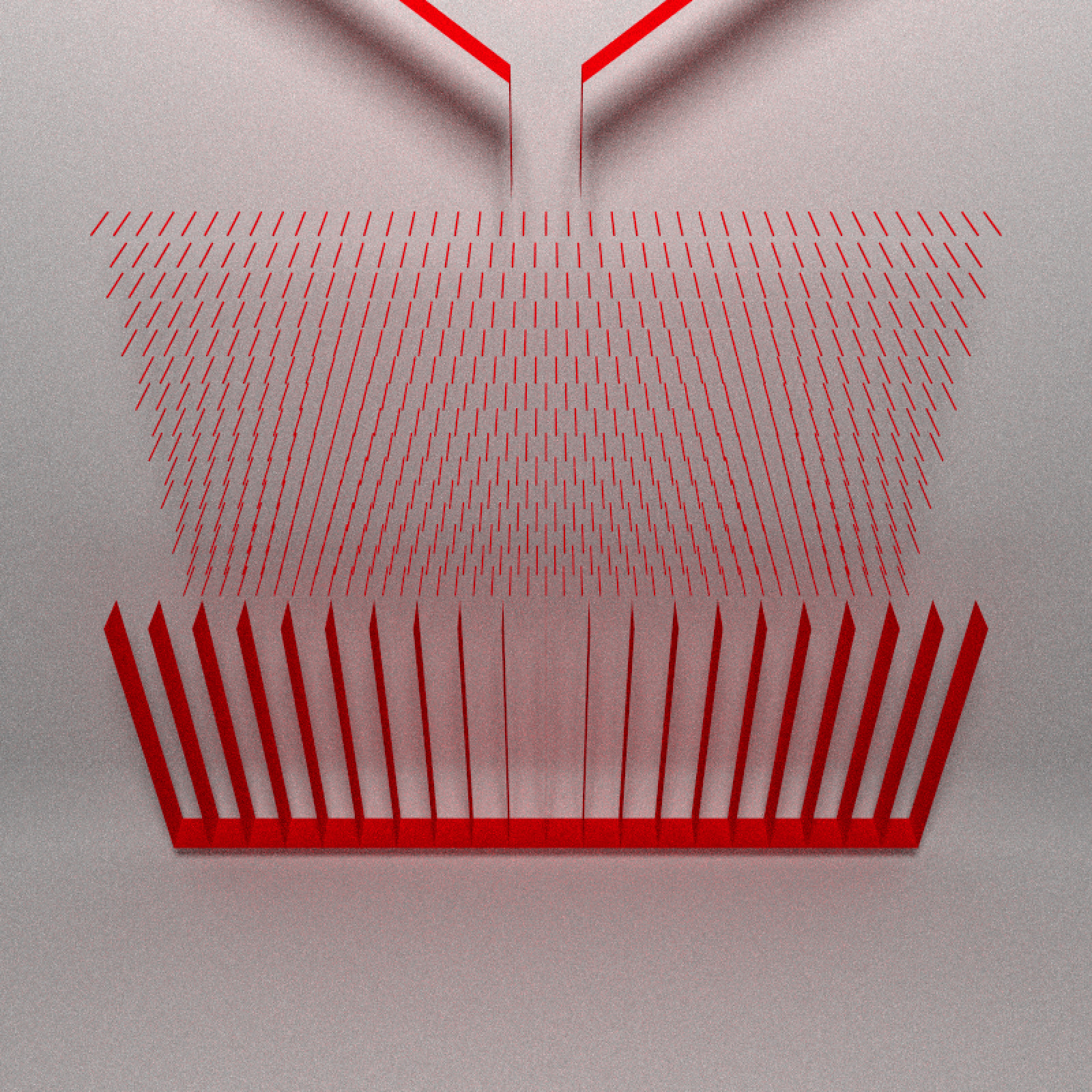
Now we have the full Galton board! We just need to throw in some balls. Let’s place 400 balls in the funnel. We scatter them randomly in a rectangular region above the spout.
cm = Chipmunk$new(time_step = 0.005)

set.seed(1)
for (i in 1:400) {
  yval = runif(1,  120, 150)
  xval = runif(1,  -20,  20)
  cm$add_circle(
    x        = runif(1,  -20,  20),
    y        = runif(1,  120, 150),
    radius   = 0.8,
    friction = 0.01
  )
}

cm$get_circles() -> balls

balllist = list()
for(i in 1:nrow(balls)) {
  balllist[[i]] = sphere(x=balls$x[i],y=balls$y[i], material = glossy(color="purple"))
}
ballscene = do.call(rbind,balllist)

generate_studio(width = 1000, height = 1000,depth=-5) %>%
  add_object(funnelscene) %>%
  add_object(pegscene) %>%
  add_object(slotscene) %>%
  add_object(ballscene) %>%
  add_object(sphere(y=150,z=150,radius=20,material=light(intensity = 40))) %>%
  render_scene(lookfrom=c(0,150,100),fov=80,lookat=c(0,80,0),samples=512,
               clamp_value = 10, sample_method = "stratified", width=800,height=800)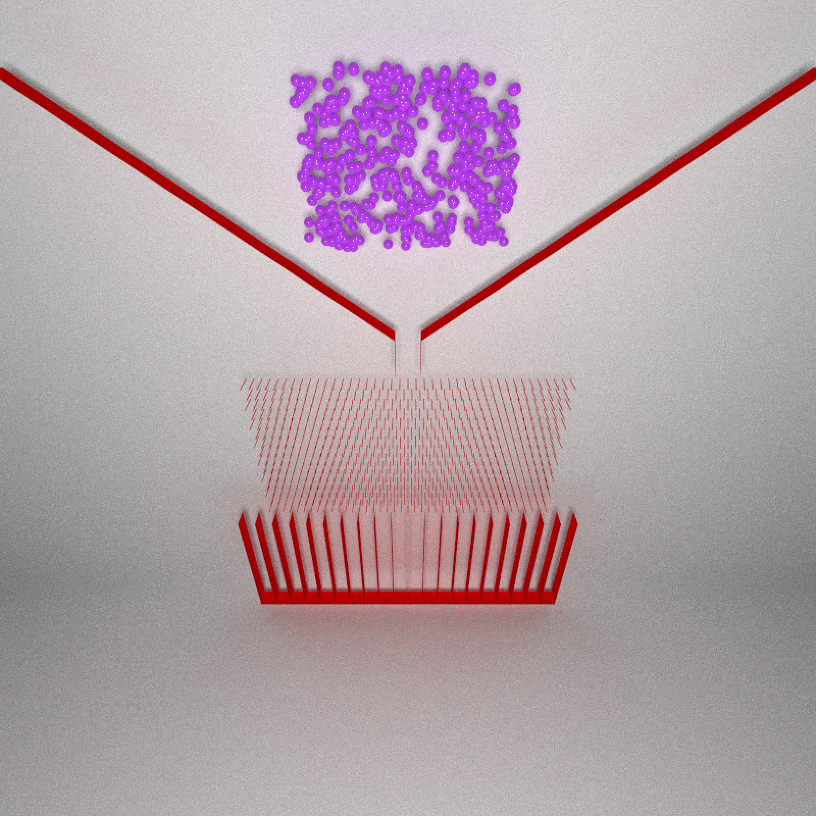
Let’s wrap all this up into a function to initialize the scene. This is so we don’t have to re-run all the above code every time we alter the board (the extra arguments angle and pout_shift we’ll use later). We’ll also include a function to extract the balls from the scene.
initialize_galton = function(cm, angle = 0, seed = 1,
                             spout_shift = 0, pegs = 15) {
  gap = 3
  cm$add_static_segment( -70 + spout_shift, 150, -gap + spout_shift, 100)
  cm$add_static_segment(  70 + spout_shift, 150,  gap + spout_shift, 100)
  cm$add_static_segment(-gap + spout_shift, 100, -gap + spout_shift,  90)
  cm$add_static_segment( gap + spout_shift, 100,  gap + spout_shift,  90)

  for (i in 1:pegs) {
    y = 90 - i * 3
    if (i %% 2 == 1) {
      xs = seq(0, 40, 2)
    } else {
      xs = seq(1, 40, 2)
    }
    xs = 1.0 * sort(unique(c(xs, -xs)))
    w = 0.05

    for (xi in seq_along(xs)) {
      xstart = xs - w * cospi(angle/180)
      xend   = xs + w * cospi(angle/180)
      cm$add_static_segment(xstart[xi],
                     y + w * sinpi(angle/180),
                     xend[xi],
                     y - w * sinpi(angle/180))
    }
  }

  floor = 85 - pegs*3 - 40
  width = 50
  for (x in seq(-width, width, 5)) {
    cm$add_static_segment(x, floor,  x,  85 - pegs * 3)
  }

  cm$add_static_segment(-width, floor, width, floor)
  cm$add_static_segment(-width, floor-0.2, width, floor-0.2)

  set.seed(seed)
  for (i in 1:400) {
    yval = runif(1,  120, 150)
    xval = runif(1,  -20,  20)
    cm$add_circle(
      x        = runif(1,  -20,  20) + spout_shift,
      y        = runif(1,  120, 150),
      radius   = 0.8,
      friction = 0.01
    )
  }
}

chipmunk_balls_to_rayrender = function(cm, color="purple") {
  cm$get_circles() -> balls
  balllist = list()
  for(i in 1:nrow(balls)) {
    balllist[[i]] = sphere(x=balls$x[i],y=balls$y[i], material = glossy(color=color))
  }
  do.call(rbind,balllist)
}
Let’s start visualizing! Here’s a snapshot at four points in the evolution of the system, where balls later in time are shifted forward in space:
cm = Chipmunk$new(time_step = 0.005)
initialize_galton(cm, seed = 2)
time1_balls = chipmunk_balls_to_rayrender(cm)
cm$advance(1000)
time2_balls = chipmunk_balls_to_rayrender(cm, color="blue")
cm$advance(1000)
time3_balls = chipmunk_balls_to_rayrender(cm, color="green")
cm$advance(1000)
time4_balls = chipmunk_balls_to_rayrender(cm, color="yellow")

generate_studio(width = 1000, height = 1000,depth=-5) %>%
  add_object(funnelscene) %>%
  add_object(pegscene) %>%
  add_object(slotscene) %>%
  add_object(group_objects(time1_balls,group_translate = c(0,0,0))) %>%
  add_object(group_objects(time2_balls,group_translate = c(0,0,20))) %>%
  add_object(group_objects(time3_balls,group_translate = c(0,0,50))) %>%
  add_object(group_objects(time4_balls,group_translate = c(0,0,75))) %>%
  add_object(sphere(y=150,z=150,radius=20,material=light(intensity = 40))) %>%
  render_scene(lookfrom=c(-180,170,200),fov=40,lookat=c(0,60,00),samples=512,
               clamp_value = 10, sample_method = "stratified", width=800,height=800)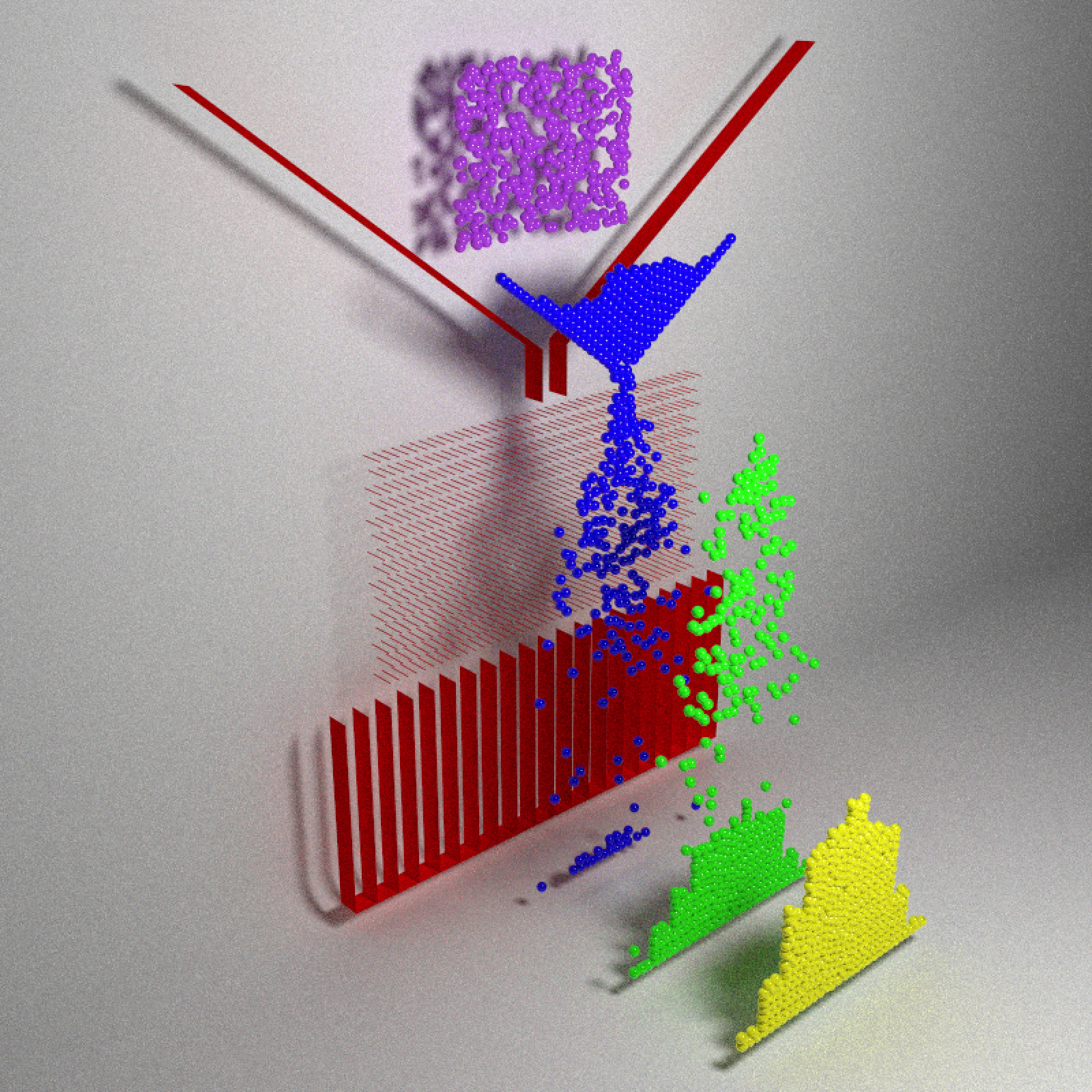
The balls fall, slowly filter through the funnel through the pegs (limited by the width of the funnel), and then finally exit out of the peg field into one of the buckets.
Changing the eed argument randomizes the initial positions, which will give us a new distribution at the bottom. We’ll use rayrender and the {av} package to create an animation visualizing the variation in these ending configurations:
ball_colors = rainbow(30)
ball_scenes = list()
for(i in 1:30) {
  cm = Chipmunk$new(time_step = 0.005)
  initialize_galton(cm, seed = i)
  cm$advance(3000)
  ball_scenes[[i]] = chipmunk_balls_to_rayrender(cm, color=ball_colors[i])
}

pegblack = generate_slot_scene(color="grey10")
slotblack = generate_slot_scene(color="grey10")
funnelblack = generate_funnel_scene(color="grey10")

#Draw normal distribution path
xvals = seq(-40, 40, length.out = 50)
yvals = dnorm(xvals,sd=15)*1700
norm_path = matrix(0,nrow=50,ncol=3)
norm_path[,1] = xvals
norm_path[,2] = yvals

for(i in 1:30) {
  generate_studio(width = 1000, height = 1000,depth=-5) %>%
    add_object(pegblack) %>%
    add_object(slotblack) %>%
    add_object(ball_scenes[[i]]) %>%
    add_object(path(norm_path,z=3,width=1,material=diffuse(color="grey10"))) %>%
    add_object(sphere(y=150,z=150,radius=50,material=light(intensity = 10))) %>%
    render_scene(lookfrom=c(-0,100,200),fov=20,lookat=c(0,20,00),samples=512,
                 filename = glue::glue("distributions{i}"),
                 clamp_value = 10, sample_method = "stratified", width=800,height=800)
}

av::av_encode_video(glue::glue("distributions{1:30}.png"),
output = "distributions.mp4", framerate = 4)We see some minor variation, but otherwise it’s a (normalish) distribution centered around zero. This is where the standard Galton demonstration usually ends: look, it’s a Gaussian distribution! Something something Central Limit Theorem. Everybody clap.
Introducing bias
=Not here though. Let’s keep on exploring. What happens when we slant each of the pegs in one direction? When a ball hits a flat peg, it’s equally likely to bounce in either direction. However, when we angle it in one direction, the ball is more likely to bounce in that direction (when striking it from above).
Let’s rotate the pegs in a circle (using the angle argument in initialize_galton()) and see what happens to the distribution. Below, I marked the theoretical center of the unbiased distribution with the purple arrow, while the actual measured center is shown with the green arrow.
angles= seq(10,360,by=10)
standard_deviations = rep(0,length(angles))
means_x = rep(0,length(angles))
arrow = rayrender::arrow

for(i in 1:length(angles)) {
  cm = Chipmunk$new(time_step = 0.005)
  initialize_galton(cm, seed = 1, angle = angles[i])
  cm$advance(3000)
  ball_angled = chipmunk_balls_to_rayrender(cm, color="red")

  means_x[i] = mean(ball_angled$x[ball_angled$shape == "sphere"])
  standard_deviations[i] = sd(ball_angled$x[ball_angled$shape == "sphere"])

  generate_studio(width = 1000, height = 1000,depth=-5) %>%
    add_object(pegblack) %>%
    add_object(slotblack) %>%
    add_object(ball_angled) %>%
    add_object(path(norm_path,z=3,width=1,material=diffuse(color="grey10"))) %>%
    add_object(arrow(start=c(means_x[i],-5,5), end = c(means_x[i],5,5),
                     radius_top = 1.5, radius=0.75,
                     material=glossy(color="purple"))) %>%
    add_object(arrow(start=c(0,-5,5), end = c(0,5,5), radius_top = 1.5, radius=0.75,
                     material=glossy(color="green"))) %>%
    add_object(sphere(y=150,z=150,radius=50,material=light(intensity = 10))) %>%
    render_scene(lookfrom=c(-0,100,200),fov=20,lookat=c(0,20,00),samples=512,
                 filename=glue::glue("bias{i}"),
                 clamp_value = 10, sample_method = "stratified", width=1200,height=800)
}

#Inset
for(i in 1:36) {
  generate_studio() %>%
    add_object(cube(xwidth=0.5,ywidth=0.1,zwidth=0.5, angle = c(0,0,angles[i]),
                    material=glossy(color="grey10"))) %>%
    add_object(sphere(y=150,z=150,radius=50,material=light(intensity = 10))) %>%
    add_object(xy_rect(z=-0.25)) %>%
    render_scene(fov=5,clamp_value=10,samples=2048,width=200,height=200,
                 min_variance = 0,
                 sample_method = "stratified",
                 filename=glue::glue("peginset{i}"))
}

library(rayimage)
for(i in 1:36) {
  temp_array = array(0,dim = c(800,1200,4))
  peg_overlay = add_title(glue::glue("peginset{i}.png"), glue::glue("Angle: {angles[i]}°"),
            title_bar_color = "black", title_color = "white",
            title_size = 18, title_position = "north", title_offset = c(0,6))
  temp_array[1:200,1:200,1:3] = peg_overlay
  temp_array[1:200,1:200,4] = 1
  add_image_overlay(glue::glue("bias{i}.png"),temp_array,filename = glue::glue("bias_with_inset{i}.png"))
}

av::av_encode_video(glue::glue("bias{1:36}.png"),
output = "bias.mp4", framerate = 4)We see the average of the distribution shifts as the pegs rotate: rotating the peg introduces bias into our system. The bias disappears when the peg is angled at multiples of 90 degrees. This is because these angles are symmetrical around the y-axis: they do not favor one direction over another. On the other hand, the bias is (approximately) largest at multiples of 45 degrees between these values. An angled peg directs downward momentum sideways, favoring one direction. We’ve now introduced an independent variable (the peg angle) that results in a shift in the mean of the distribution.
t-tests and hypothesis testing
How do we determine if it’s a significant shift? We’re using R–it’s super easy to run a t-test! We’ll use the averages and sample standard deviations we collected during the simulation. Let’s calculate our p-values/effect sizes and visualize them with a donut plot. This is a rare case where a donut plot is actually the natural method to represent the results, since our independent variable is an angle.
library(ggplot2)
library(patchwork)

pvalues = 2*pnorm(-abs(means_x/(standard_deviations/sqrt(400))))

pval_table = data.frame(angle_max=angles,angle_min=angles-10,pvalues=pvalues, means_x=means_x)

# Make the plot
p1 = ggplot(pval_table, aes(ymax=angle_max, ymin=angle_min, xmax=4, xmin=3,
                       fill=pvalues < 0.05)) +
  geom_rect() +
  coord_polar(theta="y", start = 5/180*pi, clip = "off") +
  scale_y_continuous("Peg Angle", limits=c(0,360),
                     breaks = seq(5,355,by=10),labels = c(seq(10,350,by=10),0)) +
  geom_text(aes(y=angles-5, x= 3.5, label = sprintf("%.2g",pvalues),
                angle = ifelse(angles < 180, 90-angles,-90-angles)), color = "white")+
  scale_x_continuous("",limits = c(1,4),breaks=c(1,4),labels = c("","")) +
  annotate("text",x=1,y=0,label="p-values",size=8) +
  scale_fill_manual("Reject Null\nHypothesis  \n(p < 0.05)",values = c("#bd3f00","#0486b5")) +
  theme_minimal() +
  theme(panel.grid = element_blank(),
        axis.title.x = element_text(size=18),
        axis.text.x = element_text(size=14)) +
  ggtitle("Does the Galton board distribution shift significantly for a given peg angle?")

# Make the effect size plot
p2 = ggplot(pval_table, aes(ymax=angle_max, ymin=angle_min, xmax=4, xmin=3,
                       fill=means_x)) +
  geom_rect() +
  coord_polar(theta="y", start = 5/180*pi, clip = "off") +
  scale_y_continuous("Peg Angle", limits=c(0,360),
                     breaks = seq(5,355,by=10),labels = c(seq(10,350,by=10),0)) +
  geom_text(aes(y=angles-5, x= 3.5, label = sprintf("%.2g",means_x), color = -means_x,
                angle = ifelse(angles < 180, 90-angles,-90-angles)), size=4)+
  scale_x_continuous("",limits = c(1,4),breaks=c(1,4),labels = c("","")) +
  annotate("text",x=1,y=0,label="Effect size",size=8) +
  annotate("text",x=4.5,y=45,label="P-values",size=8,angle=-45) +
  scale_fill_viridis_c("x offset") +
  scale_color_viridis_c() +
  guides(color = FALSE) +
  theme_minimal() +
  theme(panel.grid = element_blank(),
        axis.title.x = element_text(size=18),
        axis.text.x = element_text(size=14))

p1 | p2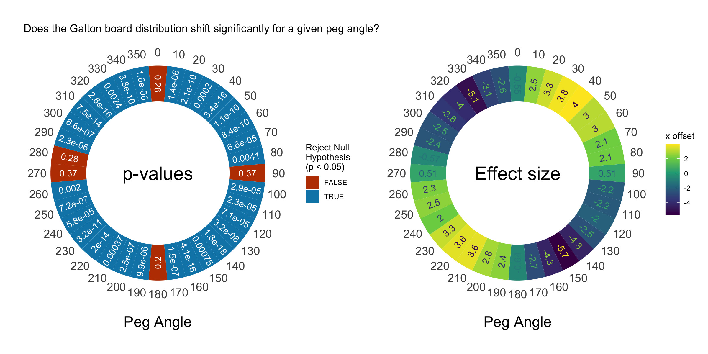
This plot shows that the distribution shifts significantly at almost every non-90 degree angle. Awesome! Now we’re demonstrating some real statistics with our Galton board. The shift is pretty small, however. Our balls are 1.6 units in diameter and our board is 100 units wide, but we only see a maximum shift of 6 units. Compared to the width of our distribution (50 units), this isn’t that big, but it’s significant.
You might now ask: is this bias introduced only from the first series of pegs, or present throughout the entire board? The top pegs are the only layers hit where the ball is more or less guaranteed to be moving straight down. Do the angled pegs continue to influence the pegs as the balls make their way through?
Bootstrapping confidence intervals + showing bias
We’ll answer these questions by looking more closely at the paths of all the balls, rather than just their final positions. Let’s extract the paths taken by a sub-sample of the balls and examine them. We’ll write a function that performs the simulation and returns the rayrender paths for a particular peg angle. We’ll then run the simulation for each 10 degree increment and show the results.
library(dplyr)

bootstrap_confidence_int = function(x) {
  boot_samples = replicate(1000, mean(sample(x, size=length(x), replace = TRUE)))
  boot_samples = boot_samples[order(boot_samples)]
  return(c(boot_samples[50],boot_samples[950]))
}

circles_to_path = function(maxtime=3000, step = 20, seed = 1,
                           angle = 0, n=5,
                           pegs = 15, spout_shift = 0, calc_mean = FALSE,
                           return_ball_coords = FALSE) {
  #initialize simulation
  cm = Chipmunk$new(time_step = 0.005)
  initialize_galton(cm, seed = seed, angle = angle, spout_shift = spout_shift, pegs = pegs)
  if(return_ball_coords) {
     cm$advance(maxtime)
    return(cm$get_circles()[1:n,])
  }
  time_val = step
  single_paths = list()
  for(i in 1:n) {
    single_paths[[i]] = list()
  }
  #Calculate position of each ball at every timestep
  counter = 1
  while(time_val < maxtime) {
    cm$advance(step)
    ball_instant = cm$get_circles()[1:n,]
    for(i in 1:n) {
      c(as.numeric(ball_instant[i,2:3]),0)
      single_paths[[i]][[counter]] = matrix(c(as.numeric(ball_instant[i,2:3]),0),ncol=3,nrow=1)
    }
    time_val = time_val + step
    counter = counter + 1
  }
  #Generate rayrender scene of all paths
  return_paths = list()
  for(i in 1:n) {
    return_paths[[i]] = path(do.call(rbind, single_paths[[i]]),width = 0.5,
                             material=glossy(color="red"))
  }
  if(calc_mean) {
    #Calculate mean x-coordinate at each y step for a single ball
    mean_paths = list()
    for(i in 1:n) {
      temp_path = as.data.frame(do.call(rbind,single_paths[[i]]))
      colnames(temp_path) = c("x","y","z")
      mean_paths[[i]] = temp_path %>%
        mutate(y = round(y)) %>%
        group_by(y) %>%
        summarise(x = mean(x)) %>%
        mutate(id = i)
    }
    all_mean_paths = dplyr::bind_rows(mean_paths)

    #Calculate mean offset and bootstrap confidence intervals
    max_y = max(all_mean_paths$y)
    min_y = min(all_mean_paths$y)
    mean_path_line = list()
    lower_ci_list = list()
    upper_ci_list = list()
    counter = 1
    for(yval in min_y:max_y) {
      single_y = all_mean_paths %>%
        filter(y == yval)
      if(nrow(single_y) > 0) {
        cis = bootstrap_confidence_int(single_y$x)
        mean_path_line[[counter]] = c(mean(unlist(single_y$x)),yval,3)
        lower_ci_list[[counter]] = c(cis[1],yval,3)
        upper_ci_list[[counter]] = c(cis[2],yval,3)
        counter = counter + 1
      }
    }
    #Add to scene
    return_paths[[n+1]] = path(mean_path_line, width=1,material=glossy(color="blue"))
    return_paths[[n+2]] = path(lower_ci_list, width=1,material=glossy(color="purple"))
    return_paths[[n+3]] = path(upper_ci_list, width=1,material=glossy(color="purple"))
  }
  dplyr::bind_rows(return_paths)
}

#Render the frames
angles= seq(10,360,by=10)

for(i in 1:36) {
  path_balls = circles_to_path(maxtime=3000, n=50, angle = angles[i], calc_mean = FALSE)
  generate_studio(width = 1000, height = 1000,depth=-5) %>%
    add_object(funnelblack) %>%
    add_object(pegblack) %>%
    add_object(slotblack) %>%
    add_object(path_balls) %>%
    add_object(sphere(y=150,z=150,radius=50,material=light(intensity = 8))) %>%
    render_scene(lookfrom=c(-0,60,200),fov=47,lookat=c(0,70,00),samples=16,
                 filename=glue::glue("ballpaths{i}"),
                 clamp_value = 10, sample_method = "stratified", width=1200,height=800)
}

for(i in 1:36) {
  temp_array = array(0,dim = c(800,1200,4))
  peg_overlay = add_title(glue::glue("peginset{i}.png"), glue::glue("Angle: {angles[i]}°"),
            title_bar_color = "black", title_color = "white",
            title_size = 18, title_position = "north", title_offset = c(0,6))
  temp_array[1:200,1:200,1:3] = peg_overlay
  temp_array[1:200,1:200,4] = 1
  add_image_overlay(glue::glue("ballpaths{i}.png"),temp_array,
                    filename = glue::glue("ballpaths_with_inset{i}.png"))
}
av::av_encode_video(glue::glue("ballpaths_with_inset{1:36}.png"),
                    output = "ballpaths_with_inset.mp4", framerate = 4)
There might be a slight pattern in the average bias, but it’s hard to tell if it’s truly shifting left or right all the way down. Let’s set the calc_mea argument in circles_to_path to TRUE to add a mean distance and bootstrapped 95% confidence intervals to our rayrender scene. If the average (x) offset grows as the balls fall through the pegs, we will say the angled pegs do bias each bounce. If the mean shifts suddenly at the top and then travels straight down, we’ll say the angled pegs only bias the first bounce, but then the randomness from the kinetic motion takes over.
I’ve increased the number of tracked balls here to 300 to get a better estimate of the mean offset. The mean is shown in blue and the 95% confidence intervals in purple. We bootstrap our 95% confidence intervals because we aren’t sure what the underlying distribution will look like. The bootstrapping process is as follows: collect all the ball positions at each (y) interval, resample at that interval with replacement and compute the mean 1000 times, order the resulting averages, and then return the 50th and 950th means in the ordered vector of averages. Let’s check it out:
for(i in 1:36) {
  path_balls = circles_to_path(maxtime=3000, n=300, angle = angles[i], calc_mean = TRUE)
  generate_studio(width = 1000, height = 1000,depth=-5) %>%
    add_object(funnelblack) %>%
    add_object(pegblack) %>%
    add_object(slotblack) %>%
    add_object(path_balls) %>%
    add_object(sphere(y=150,z=150,radius=50,material=light(intensity = 8))) %>%
    render_scene(lookfrom=c(-0,60,200),fov=47,lookat=c(0,70,00),samples=512,
                 filename=glue::glue("ball_means{i}"),verbose=TRUE,
                 clamp_value = 10, sample_method = "stratified", width=1200,height=800)
}

for(i in 1:36) {
  temp_array = array(0,dim = c(800,1200,4))
  peg_overlay = add_title(glue::glue("peginset{i}.png"), glue::glue("Angle: {angles[i]}°"),
                          title_bar_color = "black", title_color = "white",
                          title_size = 18, title_position = "north", title_offset = c(0,6))
  temp_array[1:200,1:200,1:3] = peg_overlay
  temp_array[1:200,1:200,4] = 1
  add_image_overlay(glue::glue("ball_means{i}.png"),temp_array,
                    filename = glue::glue("ballmeans_with_inset{i}.png"))
}
av::av_encode_video(glue::glue("ballmeans_with_inset{1:36}.png"),
output = "ballmeans_with_inset.mp4", framerate = 4)We can see here that the line shifts in one direction as the balls travel through the board–the pegs do continue to influence the direction of each bounce. It’s not just an offset from the first step of pegs. Our bootstrapped confidence intervals show us that the variation in position grows as the balls fall through the board. The blue line shows how the center of the distribution shifts as the balls travel through the angled pegs. The total bias grows with the length of the board. This brings us to our next Galton board lesson: interaction effects!
Interaction effects
What do I mean when I write “interaction effects”? Let’s see the effect of changing the number of pegs at a fixed peg angle. We’ll visualize boards with 1 layer, 15 layers, and 30 layers:
peg_1_scene = generate_peg_scene(pegs=1, color="grey10")
slot_1_scene = generate_slot_scene(pegs=1, color="grey10")
path_1peg_balls = circles_to_path(maxtime=3000, n=300,
                             angle = 45,
                             pegs = 1,
                             calc_mean = TRUE)

peg_15_scene = generate_peg_scene(pegs=15, color="grey10")
slot_15_scene = generate_slot_scene(pegs=15, color="grey10")
path_15peg_balls = circles_to_path(maxtime=3000, n=300,
                             angle = 45,
                             pegs = 15,
                             calc_mean = TRUE)

peg_30_scene = generate_peg_scene(pegs=30, color="grey10")
slot_30_scene = generate_slot_scene(pegs=30, color="grey10")
path_30peg_balls = circles_to_path(maxtime=3000, n=300,
                             angle = 45,
                             pegs = 30,
                             calc_mean = TRUE)

par(mfrow=c(1,3))
generate_studio(width = 1000, height = 1000,depth=-200) %>%
  add_object(funnelblack) %>%
  add_object(peg_1_scene) %>%
  add_object(slot_1_scene) %>%
  add_object(path_1peg_balls) %>%
  add_object(sphere(y=150,z=150,radius=50,material=light(intensity = 8))) %>%
  render_scene(lookfrom=c(-0,60,200),fov=47,lookat=c(0,30,00),samples=512,
               clamp_value = 10, sample_method = "stratified", width=400,height=600)

generate_studio(width = 1000, height = 1000,depth=-200) %>%
  add_object(funnelblack) %>%
  add_object(peg_15_scene) %>%
  add_object(slot_15_scene) %>%
  add_object(path_15peg_balls) %>%
  add_object(sphere(y=150,z=150,radius=50,material=light(intensity = 8))) %>%
  render_scene(lookfrom=c(-0,60,200),fov=47,lookat=c(0,30,00),samples=512,
               clamp_value = 10, sample_method = "stratified", width=400,height=600)

generate_studio(width = 1000, height = 1000,depth=-200) %>%
  add_object(funnelblack) %>%
  add_object(peg_30_scene) %>%
  add_object(slot_30_scene) %>%
  add_object(path_30peg_balls) %>%
  add_object(sphere(y=150,z=150,radius=50,material=light(intensity = 8))) %>%
  render_scene(lookfrom=c(-0,60,200),fov=47,lookat=c(0,30,00),samples=512,
               clamp_value = 10, sample_method = "stratified", width=400,height=600)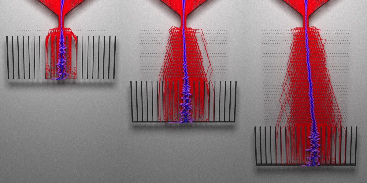
A single layer of angled pegs does not significantly bias the distribution, even though the angle I used (45 degrees) is supposed to result in the largest effect size. When we increase the depth of the board, the bias grows. The peg angle is actually an interaction effect: the effect size depends on both the board length and the angle. Varying just the board length does not bias the distribution, nor does just changing the peg angle by itself. The effect depends on a combination of the two factors.
We can see this explicitly if we fit a model. Let’s extract the ball coordinates for different inputs and fit a linear model to see what terms are significant. We’ll also shift the spout position left and right, which we know will shift the center of the distribution.
par(mfrow=c(1,1))
board_factors = expand.grid(angles = c(-45,45),
                            peg_depth = c(1,31),
                            spout = c(-2,2))

ball_coords_model = list()
for(i in 1:nrow(board_factors)) {
  ball_coords_model[[i]] = circles_to_path(maxtime=3000, n=300,
                  spout_shift = board_factors$spout[i],
                  angle = board_factors$angles[i],
                  pegs = board_factors$peg_depth[i],return_ball_coords = TRUE)
  ball_coords_model[[i]]$angle =  board_factors$angles[i]
  ball_coords_model[[i]]$peg_depth =  board_factors$peg_depth[i]
  ball_coords_model[[i]]$spout =  board_factors$spout[i]
}
all_peg_data = do.call(rbind,ball_coords_model)

fit = lm(data = all_peg_data, x ~ (angle + peg_depth + spout)^3)
summary(fit)
## Call:
## lm(formula = x ~ (angle + peg_depth + spout)^3, data = all_peg_data)
##
## Residuals:
## Min 1Q Median 3Q Max
## -247.135 -6.622 -0.013 6.832 39.646
##
## Coefficients:
## Estimate Std. Error t value Pr(>|t|)
## (Intercept) -0.0118719 0.3349737 -0.035 0.972
## angle 0.0001362 0.0074439 0.018 0.985
## peg_depth 0.0136698 0.0152735 0.895 0.371
## spout 1.0035564 0.1674868 5.992 2.39e-09 ***
## angle:peg_depth 0.0051148 0.0003394 15.070 < 2e-16 ***
## angle:spout 0.0014254 0.0037219 0.383 0.702
## peg_depth:spout 0.0079628 0.0076367 1.043 0.297
## angle:peg_depth:spout -0.0002158 0.0001697 -1.271 0.204
## ---
## Signif. codes: 0 '***' 0.001 '**' 0.01 '*' 0.05 '.' 0.1 ' ' 1
##
## Residual standard error: 11.22 on 2392 degrees of freedom
## Multiple R-squared: 0.1973, Adjusted R-squared: 0.195
## F-statistic: 83.99 on 7 and 2392 DF, p-value: < 2.2e-16
Now it’s official! When the full model is fit, neither the angle nor the depth are significant on their own, but the interaction between the two is significant. Our other significant term is the spout position, which is obvious: move the spout left or right and the resulting distribution will also shift in the same direction. The parameter estimates illustrate this: a one unit shift in spout position results in a 1.00 ± 0.16 unit shift in the distribution, which shows the center of the distribution exactly follows the shift in the spout.
The angle:peg_depth effect is more subtle: a 1 unit increase in depth increases the effect of changing the angle by 0.005 ± 0.0003 units. Interactions are a bit more tricky to interpret than main effects. You aren’t shifting the distribution directly; an interaction instead augments the size of the main effect. To see this more clearly, let’s look at our model (3 main effects + 1 interaction):
We can rearrange this to show how the interaction can be interpreted as changing the main effect term:
\[y = \beta_0 + (\beta_{1} + \beta_{12}x_2) x_1 + \beta_{2} x_2 + \beta_{3} x_3 + \epsilon\]Equivalently, we could also say the interaction term is augmenting the \(\beta_2\) term: these interpretations are mathematically equivalent:
\[y = \beta_0 + \beta_{1} x_1 + (\beta_{2} + \beta_{12}x_1) x_2 + \beta_{3} x_3 + \epsilon\]All this to say: look, we’ve demonstrated a non-trivial linear regression with a Galton board! Way more interesting than the Central Limit Theorem.
Conclusion
I hope you enjoyed this deeper-than-usual dive into the mechanics of a customizable Galton board. When you have full control of how one is built, a Galton board can be a fruitful toy model to demonstrate different statistical concepts. Here are some other questions you might consider investigating on your own:
- Is the distribution of balls truly normal? Is there a good way to test this?
- What happens to the distribution when you decrease/increase the bucket size?
- What happens to the distribution when you decrease/increase the number of balls?
- What happens to the distribution when you make the spout gap wider/narrower?
- Is there a way to change the board to generate other distributions?
- Does changing the elasticity of the balls affect the variance of the resulting distribution?
Thanks to @coolbutuseless for creating the chipmunkcore/chipmunkbasic packages that made all this possible! If you’re interested in learning more about the package used to render these 3D visualizations, check out the package website:
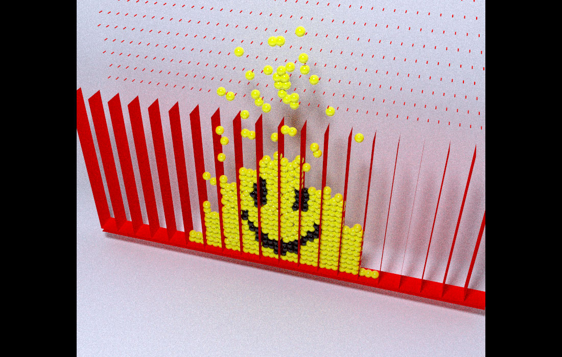
One last question–how did you get the smiley face in the Galton board animation?
It’s deceptively simple: we run the simulation and find the final positions of the balls. Then we record the IDs of the balls that fall into the areas we want to color black. Then we reverse time (by resetting the random seed) and run the simulation over again, but this time color those balls black from the beginning.
cm = Chipmunk$new(time_step = 0.005)

initialize_galton(cm)
cm$advance(3000)
cm$get_circles() -> balls

#Find ball IDs that end up in the mouth and eyes and save them
smile_balls = list()
for(i in 1:nrow(balls)) {
  if((balls$x[i] * balls$x[i]+60 >  balls$y[i]*10 &
      balls$x[i] * balls$x[i]+20 <  balls$y[i]*10 &
      balls$x[i] < 10 &  balls$x[i] > -10) |
     ((balls$x[i] - 5)*2)^2 +  (balls$y[i] - 20)^2 < 4^2 |
     ((balls$x[i] + 5)*2)^2 +  (balls$y[i] - 20)^2 < 4^2) {
    smile_balls[[i]] = balls$idx[i]
  }
}

idvals = unlist(smile_balls)

#Re-run simulation and render animation
cm <- Chipmunk$new(time_step = 0.005)
initialize_galton(cm)

fovvec = seq(90,30,length.out = 600)
yvec = (unlist(tweenr::tween(c(50,20),n=600)))

for (j in 1:600) {
  cm$advance(5)
  cm$get_circles() -> balls

  #Color balls
  balllist = list()
  for(i in 1:nrow(balls)) {
    if(balls$idx[i] %in% idvals) {
      balllist[[i]] = sphere(x=balls$x[i],y=balls$y[i], material = glossy(color="black"))
    } else {
      balllist[[i]] = sphere(x=balls$x[i],y=balls$y[i], material = glossy(color="yellow"))
    }
  }
  balls = do.call(rbind,balllist)

  generate_studio(width = 1000, height = 1000,depth=-5) %>%
    add_object(funnelscene) %>%
    add_object(pegscene) %>%
    add_object(slotscene) %>%
    add_object(balls) %>%
    add_object(sphere(y=200,z=100,radius=20,material=light(intensity = 40))) %>%
    render_scene(lookfrom=c(30,100,100),fov=fovvec[j],lookat=c(0,yvec[j],0),samples=128,
                 clamp_value = 10,filename=glue::glue("galtonanim{j}"),
                 sample_method = "stratified", width=800,height=800)
}

av::av_encode_video(glue::glue("galtonanim{1:600}.png"),
                    output = "galtonanim.mp4", framerate = 60)