Raybonsai: Generate Procedural 3D Trees in R
One fun aspect of building a 3D renderer in R (and more generally, building anything in a programming language with a REPL) is the lack of friction between your code your results: rather than constructing a 3D scene by hand using a GUI, you can generate your scene directly from data or purely from logic. For traditional 3D rendering, this isn’t particularly useful, but for visualizing data and procedurally-generated systems, this close link allows for fast iteration and reproducibility.
Rayrender was built around this idea: instead of trying to integrate an external renderer into the R ecosystem (which is difficult for many reasons, primarily CRAN requirements), it made sense to build a 3D renderer designed specifically for R. There’s one big hurdle you encounter when writing your own software, however: in the beginning, there is no one but you who knows how to use it! “If you build it, they will come” is not a viable strategy for software. Regardless of how useful you think your package/application is, few people are going to take the time to learn it unless they’re presented with motivating examples. So, with that in mind, I’m always on the lookout for interesting and novel visualization ideas that will give people a better idea of what rayrender is capable of, and hopefully inspire them to experiment with the software.
What does all this have to do with 3D trees? Back in April, Danielle Navarro released an the flametree package, which produces procedural 2D trees using a stochastic L-system, and I thought: I think these would look really cool in 3D! So I dove into her code. It wasn’t too difficult to generalize it to 3D, write a layer that translated the resulting data structure into rayrender’s tibble-based scene format using rayrender primitives, and package it all up for easy installation. And that brings us to…
The raybonsai package! A package that creates and renders procedural 3D trees in R. Installation is easy: just use the remote package to install from Github:
emotes::install_github("tylermorganwall/raybonsai")
There are currently only two user-facing functions in raybonsai: generate_tree() and render_tree(). generate_tree() generates a tree that follows a certain set of constraints that you set and returns a rayrender scene describing the tree. render_tree() automatically adds ground, sets up lighting, and sets up the camera so the tree is in frame, but is otherwise just a light wrapper around rayrender’s render_scene() function.
Let’s try it out, with the default settings:
library(raybonsai)

generate_tree() %>%
  render_tree()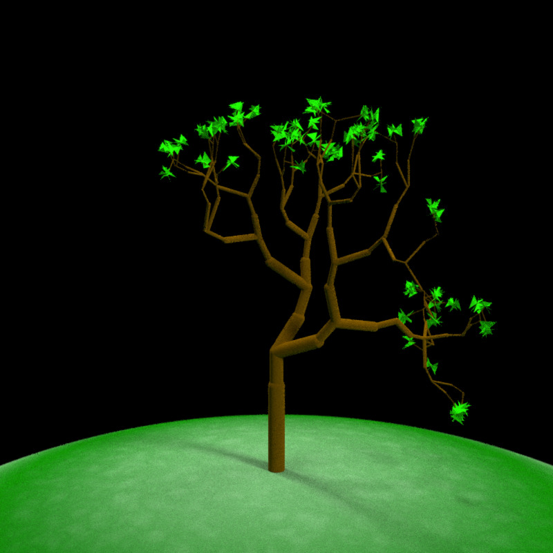
A tree! Let’s customize it. The growth of the tree is controlled primarily using five inputs: the number of branches at each branching point branch_split, the horizontal branching angle branch_angle, the vertical branching angle branch_angle_vert, the scaled length of each subsequent branch branch_scale, and (most appropriately named, given the use case) the random seed seed. Let’s first start by generating a bunch of different plants, each with the same settings but different seeds.
par(mfrow=c(3,3))
for(i in 1:9) {
  generate_tree(seed = i) %>%
    render_tree()
}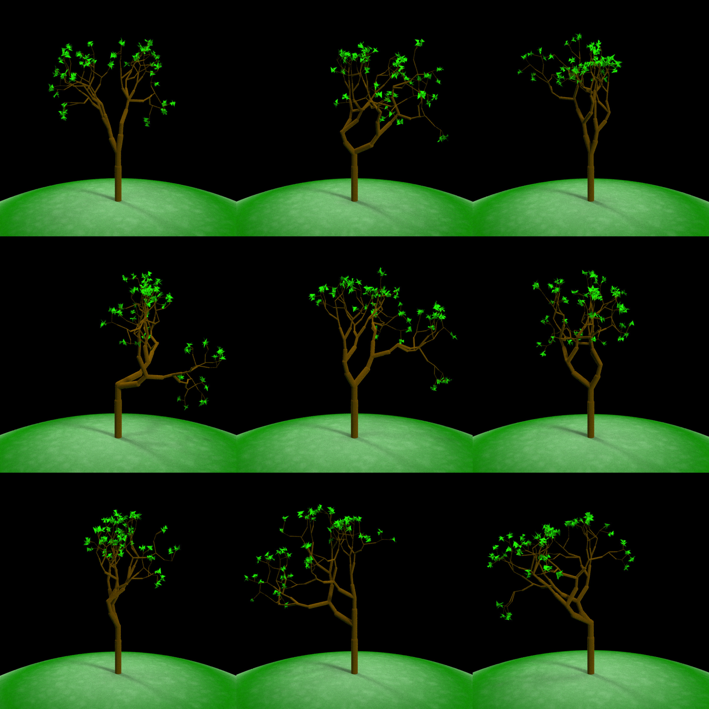
Each tree is different, but they all appear to come from the same “species.” And that’s because they’re all generated using the same “DNA”: the branch angles and scaling factors. Let’s change that DNA by specifying a new set of rules. Here, we cut the potential angles the branches can make from -45 and 45 degrees in half:
par(mfrow=c(3,3))
for(i in 1:9) {
  generate_tree(seed = i, branch_angle_vert = seq(-45,45,by=5)/2, leaf_color = "pink") %>%
    render_tree()
}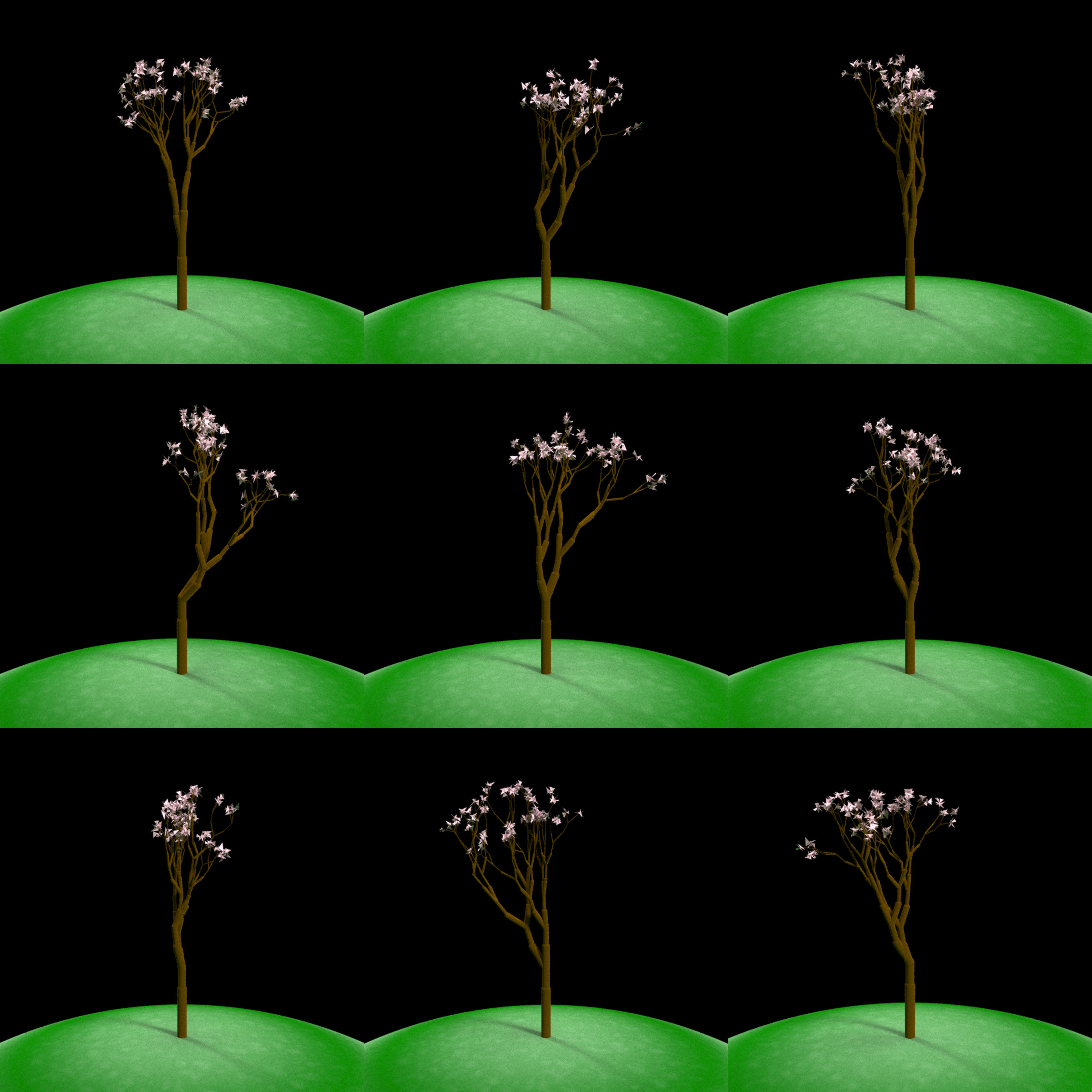
These are visually quite distinct from the previous batch and have a similar appearance to each other. But look closely and compare these trees with the first batch: you’ll see that they actually have the exact same branching structure, just with less pronounced branching angles (note the trees than lean left/right in the first batch still lean that way in the second). This is because the random choice whether to branch left or right is controlled by the random seed, which is identical between the two batches. The only variable that’s different is the branching angle itself.
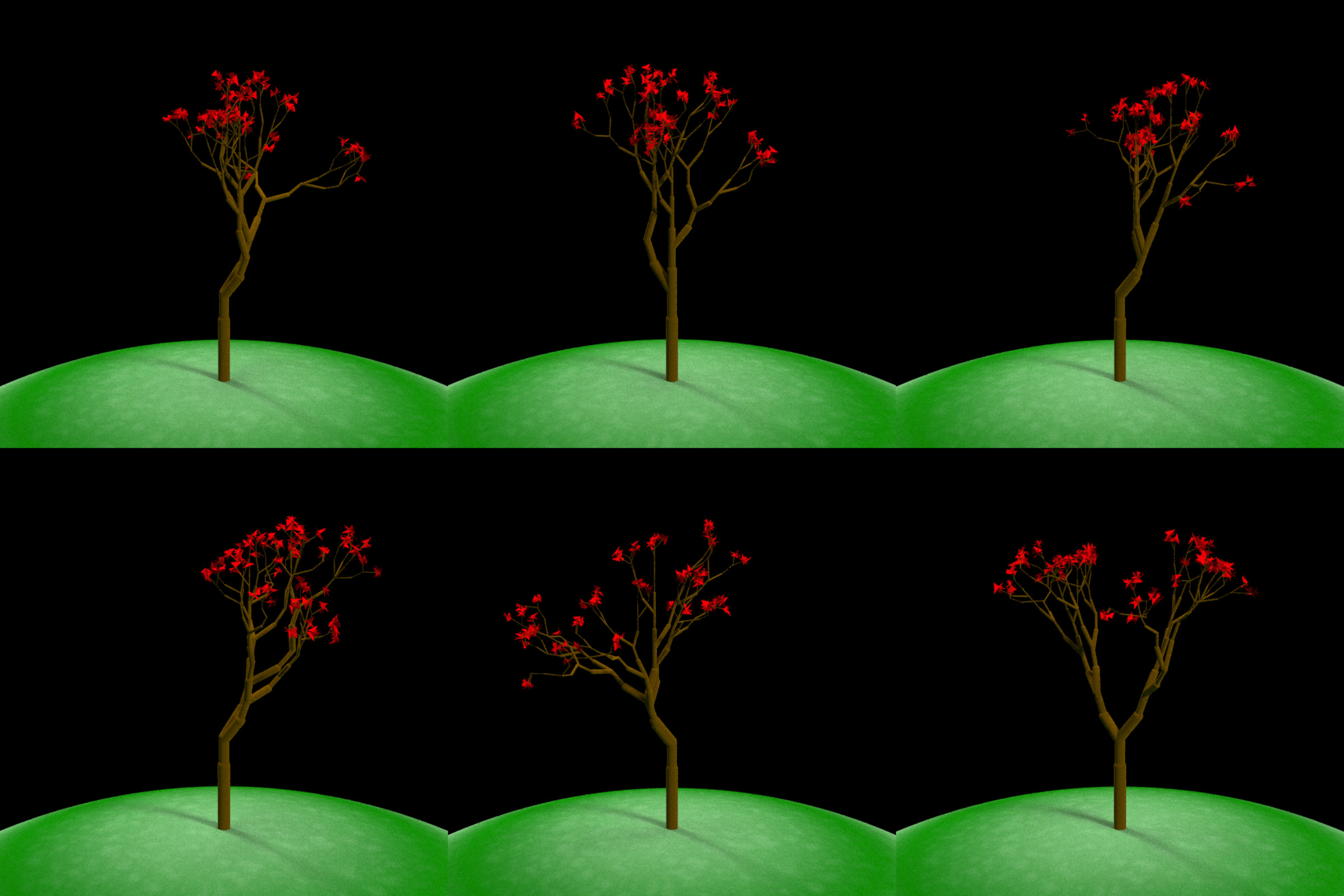
What happens when we add an addition angle into the mix? Here, one directly in the center. Now, each branch can either go left, right, or continue in the same direction as the source branch. We can see this results in some trees developing “trunks” and some longer straight branches:
par(mfrow=c(2,3))
for(i in 1:6) {
  generate_tree(seed = i, branch_angle_vert = c(-20,0, 20), leaf_color = "red") %>%
    render_tree()
}
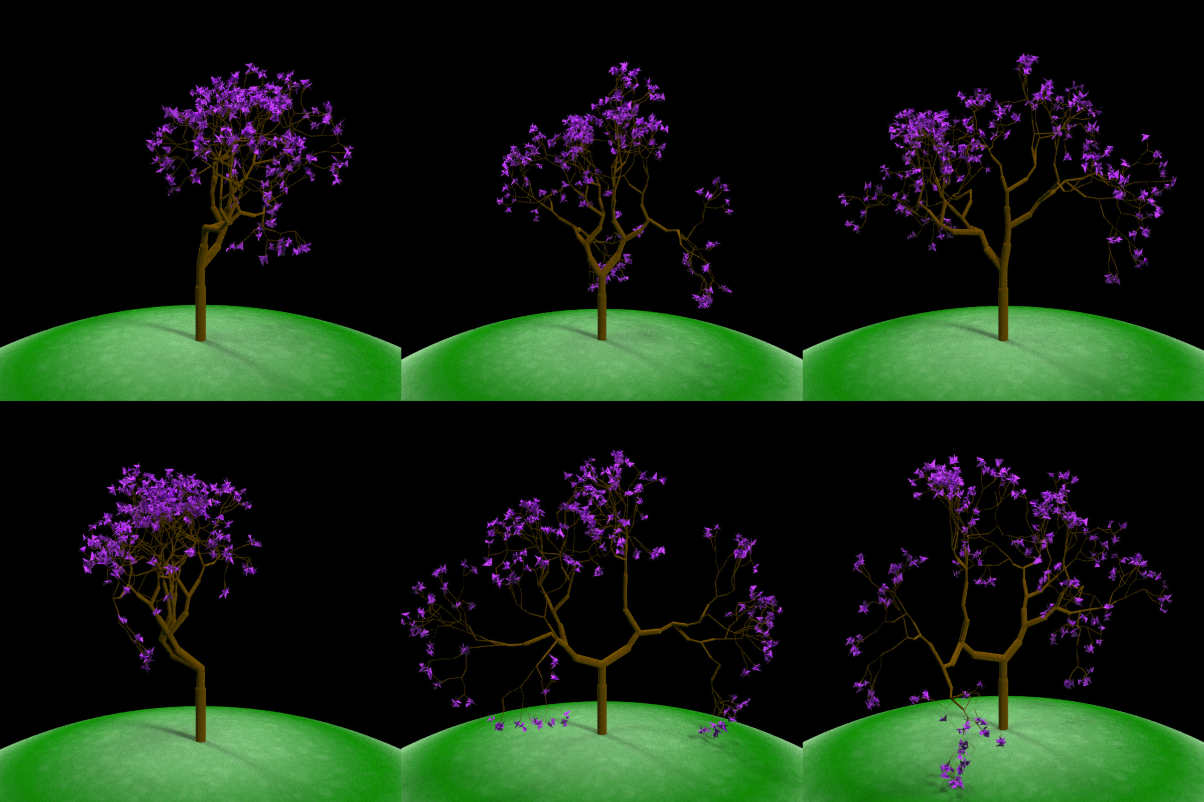
The next variable we can control is increase the branching depth of the tree. By default, we generate 6 branch layers. The number of branches grows exponentially with each layer, so we’ll just increase it to 8. This will increase the visual complexity of our tree.
par(mfrow=c(2,3))
for(i in 1:6) {
  generate_tree(seed = i+1000, branch_depth = 8, leaf_color = "purple") %>%
    render_tree()
}
By default, raybonsai only adds leaves to the last layer, but we can start growing them on earlier layers to fill in our tree:
par(mfrow=c(1,2))

generate_tree(seed = 1234, branch_depth = 8, leaf_color = "orange") %>%
  render_tree()

generate_tree(seed = 1234, branch_depth = 8, leaf_color = "orange", leaf_depth_start = 5) %>%
  render_tree()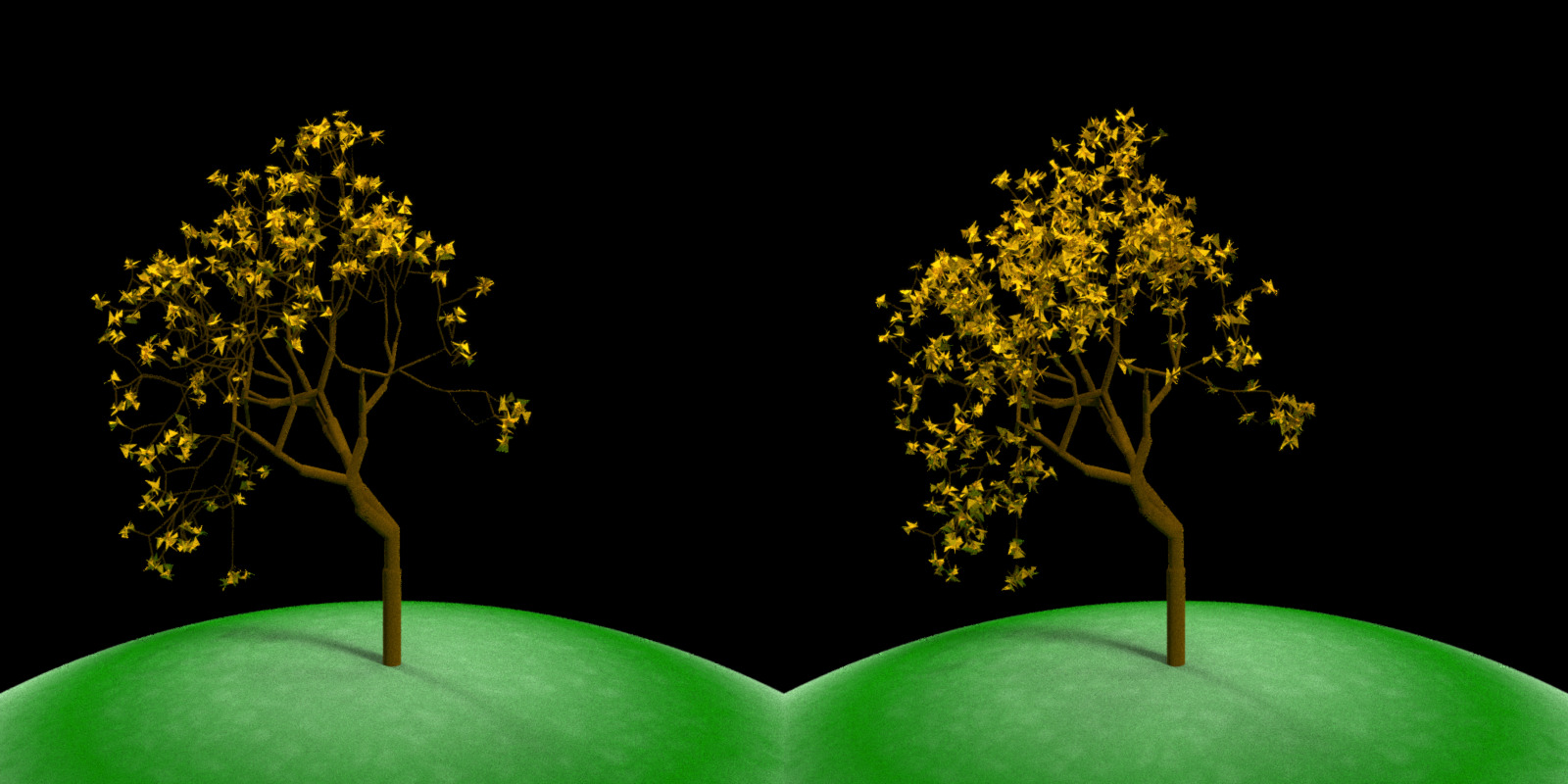
Up to this point, we’ve kept the trees symmetric by setting a matching negative angle for every positive angle. We can also make asymmetric trees by increasing the probability that we’ll select one angle over another. Here each branch has a 5x probability of turning one way versus the other, implemented by duplicating one angle 5x in the branching vector.
par(mfrow=c(1,2))
generate_tree(seed = 2020, branch_angle_vert = c(-10, 10, 10, 10, 10, 10),
              branch_depth = 8, leaf_color = "magenta", leaf_depth_start = 5) %>%
  render_tree()
generate_tree(seed = 2021, branch_angle_vert = c(10,-10,-10,-10,-10,-10),
              branch_depth = 8, leaf_color = "magenta", leaf_depth_start = 5) %>%
  render_tree()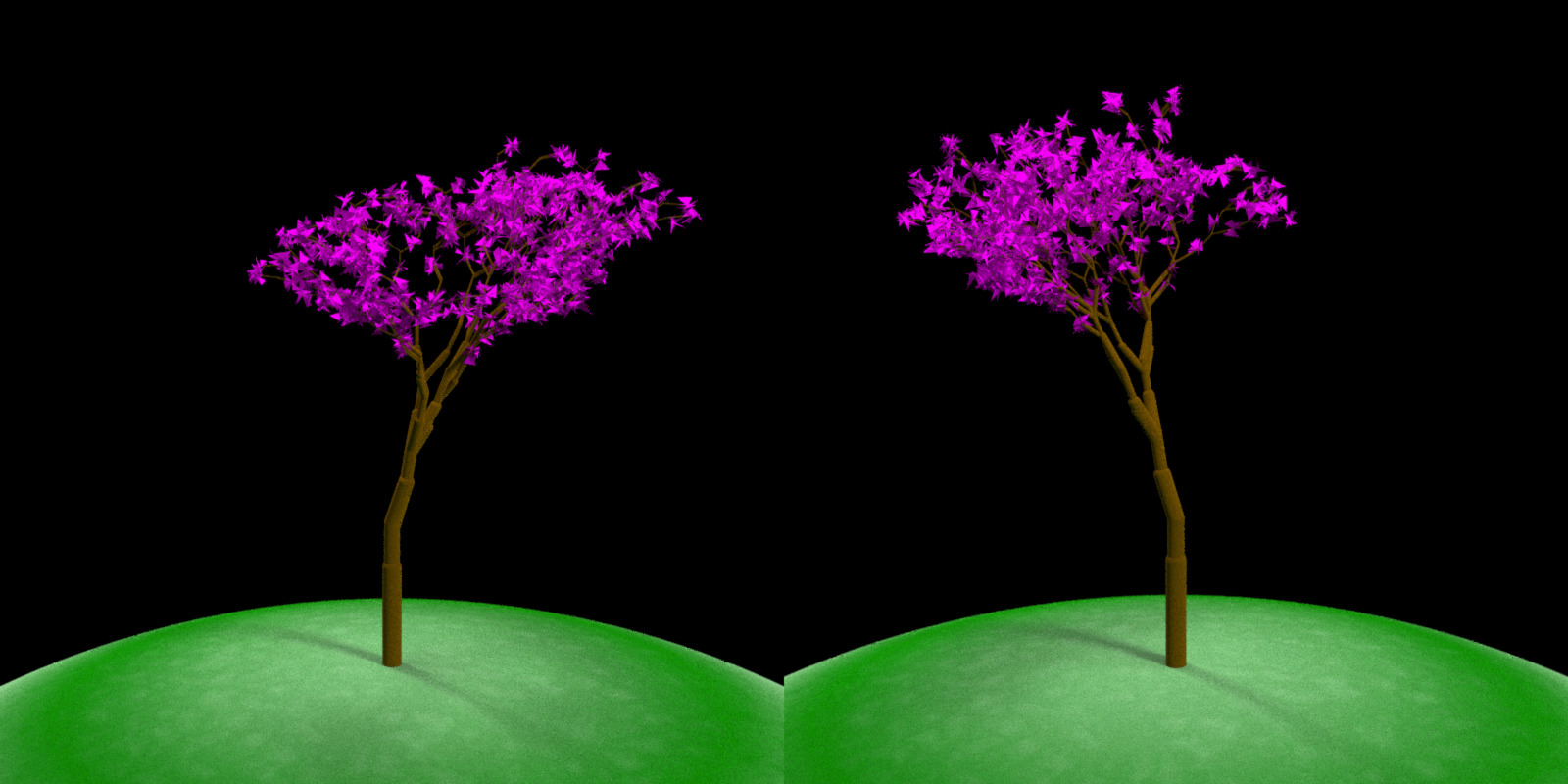
We can also create asymmetric trees by ensuring the average angle is negative or positive, without repeating individual angles. This works because on average, the tree favors one direction over the other.
par(mfrow=c(1,2))
generate_tree(seed = 4321, branch_angle_vert = seq(-10,20,by=1),
              branch_depth = 8, leaf_color = "yellow", leaf_depth_start = 5) %>%
  render_tree()

generate_tree(seed = 4321, branch_angle_vert = -seq(-10,20,by=1),
              branch_depth = 8, leaf_color = "yellow", leaf_depth_start = 5) %>%
  render_tree()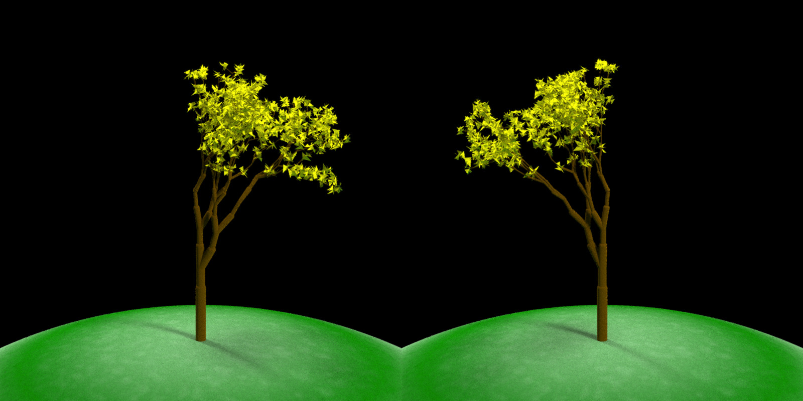
Another variable we can control is the scaling factor branch_scale, which defaults to c(0.8, 0.9) (meaning each branch is either 80% or 90% the length of the previous layer). If we decrease or increase this, the resulting tree will be dramatically different:
par(mfrow=c(1,3))
generate_tree(seed = 10, branch_angle = c(-30,0, 30), branch_scale = c(0.6,0.7),
              branch_depth = 7, leaf_color = "green", leaf_depth_start = 5) %>%
  render_tree()

generate_tree(seed = 11, branch_angle = c(-30,0, 30), branch_scale = c(0.9,1),
              branch_depth = 7, leaf_color = "green", leaf_depth_start = 5) %>%
  render_tree()

generate_tree(seed = 12, branch_angle = c(-30,0, 30), branch_scale = c(1.1,1.2),
              branch_depth = 7, leaf_color = "green", leaf_depth_start = 5) %>%
  render_tree()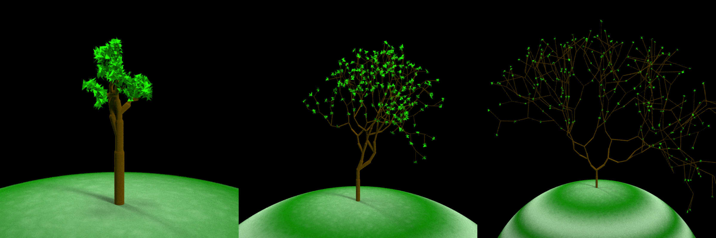
Each tree so far has been grown with the “midpoint” method: rather than growing each branch from the end of the previous branch, the default behavior extends the branch in the previous branches direction until it reaches the halfway point, and only then extends a branch to the endpoint. We can turn off this feature and by setting midpoint = FALSE: This results in a structurally identical tree with a slightly different appearance. And for fun, let’s also play around with the ground color and the branch color:
par(mfrow=c(1,2))
generate_tree(seed = 20, branch_angle = c(-30,0, 30), branch_scale = c(0.9,1), midpoint = TRUE,
              branch_depth = 7, leaf_color = "chartreuse4",
              leaf_depth_start = 5, branch_color = "tan") %>%
  render_tree(ground_color1 = "darkgoldenrod4", ground_color2 = "chocolate4")

generate_tree(seed = 20, branch_angle = c(-30,0, 30), branch_scale = c(0.9,1), midpoint = FALSE,
              branch_depth = 7, leaf_color = "chartreuse4",
              leaf_depth_start = 5, branch_color = "tan") %>%
  render_tree(ground_color1 = "darkgoldenrod4", ground_color2 = "chocolate4")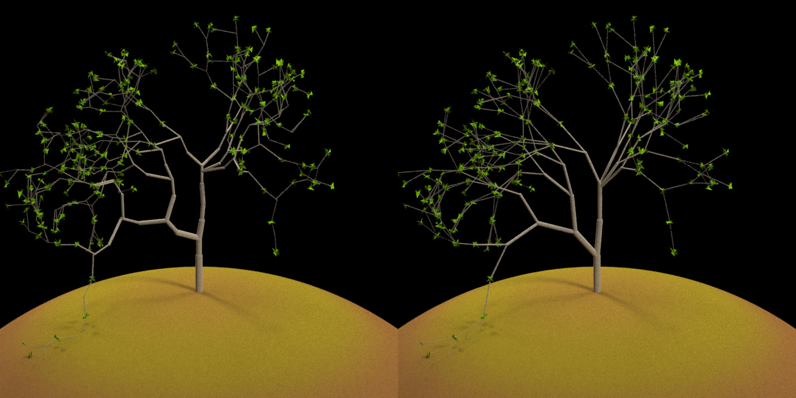
The lighting here is automatically set up by render_tree(), but we can turn it off and set up our own lighting using rayrender. We’ll also set branch_split = 3 here for a denser tree with more branches:
library(rayrender)

par(mfrow=c(1,1))
generate_tree(seed = 222, branch_angle = c(-20, 20), branch_scale = c(0.8,0.9), branch_split = 3,
              branch_depth = 6 , leaf_color = "chartreuse4",
              leaf_depth_start = 5, branch_color = "tan") %>%
  add_object(sphere(x=5,y=1,radius=1,material=light(color="magenta",intensity = 30))) %>%
  add_object(sphere(x=-5,y=1,radius=1,material=light(color="dodgerblue",intensity = 30))) %>%
  raybonsai::render_tree(lights = FALSE, ground_color1 = "grey50",ground_color2 = "grey50", width=1200,height=800)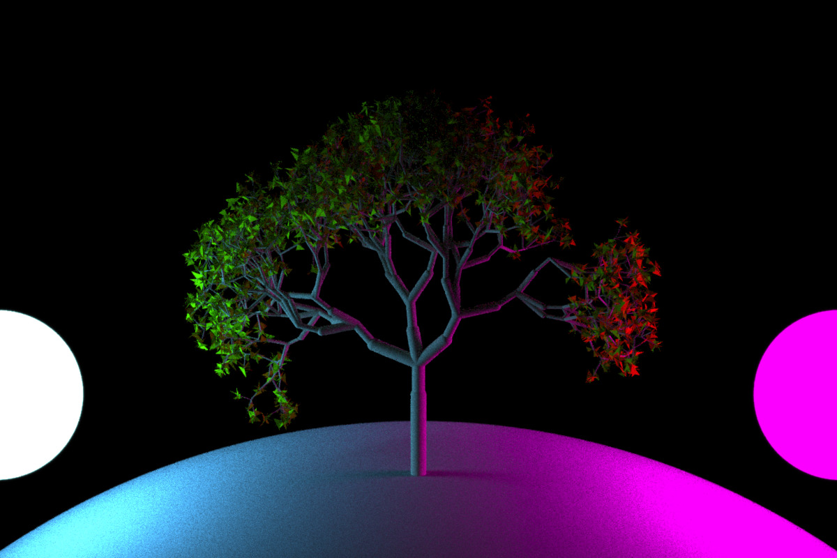
We can also load an HDR image (here, obtained for free from hdrihaven.com) to light the scene with realistic lighting:
generate_tree(seed = 222, branch_angle = c(-20,20), branch_scale = c(0.8,0.9),
              branch_depth = 10 , leaf_color = "chartreuse4",
              leaf_depth_start = 5, branch_color = "tan") %>%
  raybonsai::render_tree(lights = FALSE, environment_light = "kiara_3_morning_2k.hdr", width=1200, height=800)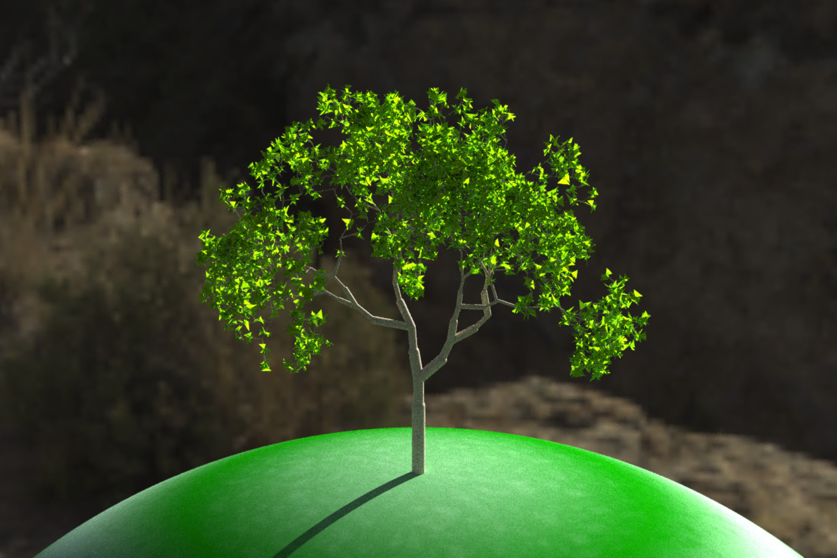
We can even add multiple trees by using rayrender’s group_objects() function to rotate them around the ground (here a sphere centered at y = -10).
tree1 = generate_tree(seed = 1111, branch_angle_vert = c(-45,0,45),
              branch_depth = 8 , leaf_color = "green", leaf_depth_start = 5)
tree2 = generate_tree(seed = 2222, branch_angle_vert = seq(-30,30,by=5),
              branch_depth = 8 , leaf_color = "red", leaf_depth_start = 5)
tree3 = generate_tree(seed = 3333, branch_angle_vert = seq(-30,30,by=5),
              branch_depth = 8 , leaf_color = "purple", leaf_depth_start = 5)
tree4 = generate_tree(seed = 4444, branch_angle_vert = c(-45,0,45),
              branch_depth = 8 , leaf_color = "orange", leaf_depth_start = 5)

group_objects(tree1,pivot_point = c(0,-10,0), group_angle = c(0,0,10)) %>%
  add_object(group_objects(tree2,pivot_point = c(0,-10,0), group_angle = c(0,0,30))) %>%
  add_object(group_objects(tree3,pivot_point = c(0,-10,0), group_angle = c(0,0,-10))) %>%
  add_object(group_objects(tree4,pivot_point = c(0,-10,0), group_angle = c(0,0,-30))) %>%
  raybonsai::render_tree(lights = FALSE, environment_light = "noon_grass_2k.hdr",
                         samples=40,
              aperture=0.5, fov=24, lookfrom=c(0,8,30), width=1200, height=800,
              ground_color1 = "darkgreen", ground_color2 = "darkgreen")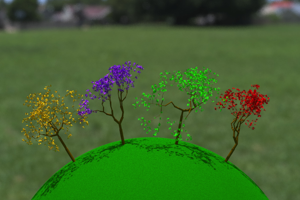
render_tree() allows us to manually change the camera position and direction to focus on certain regions of interest by passing lookat and lookfrom arguments:
group_objects(tree1,pivot_point = c(0,-10,0), group_angle = c(0,0,10)) %>%
  add_object(group_objects(tree2,pivot_point = c(0,-10,0), group_angle = c(0,0,30))) %>%
  add_object(group_objects(tree3,pivot_point = c(0,-10,0), group_angle = c(0,0,-10))) %>%
  add_object(group_objects(tree4,pivot_point = c(0,-10,0), group_angle = c(0,0,-30))) %>%
  render_tree(lights = FALSE, environment_light = "noon_grass_2k.hdr",
              fov=8, lookat=c(-2,3,0),lookfrom=c(20,2,30),
              aperture=1, width=1200, height=800,
              ground_color1 = "darkgreen", ground_color2 = "darkgreen")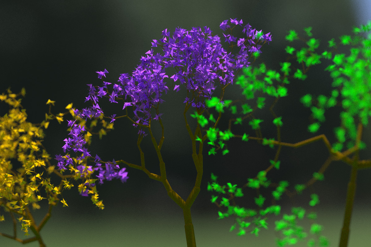
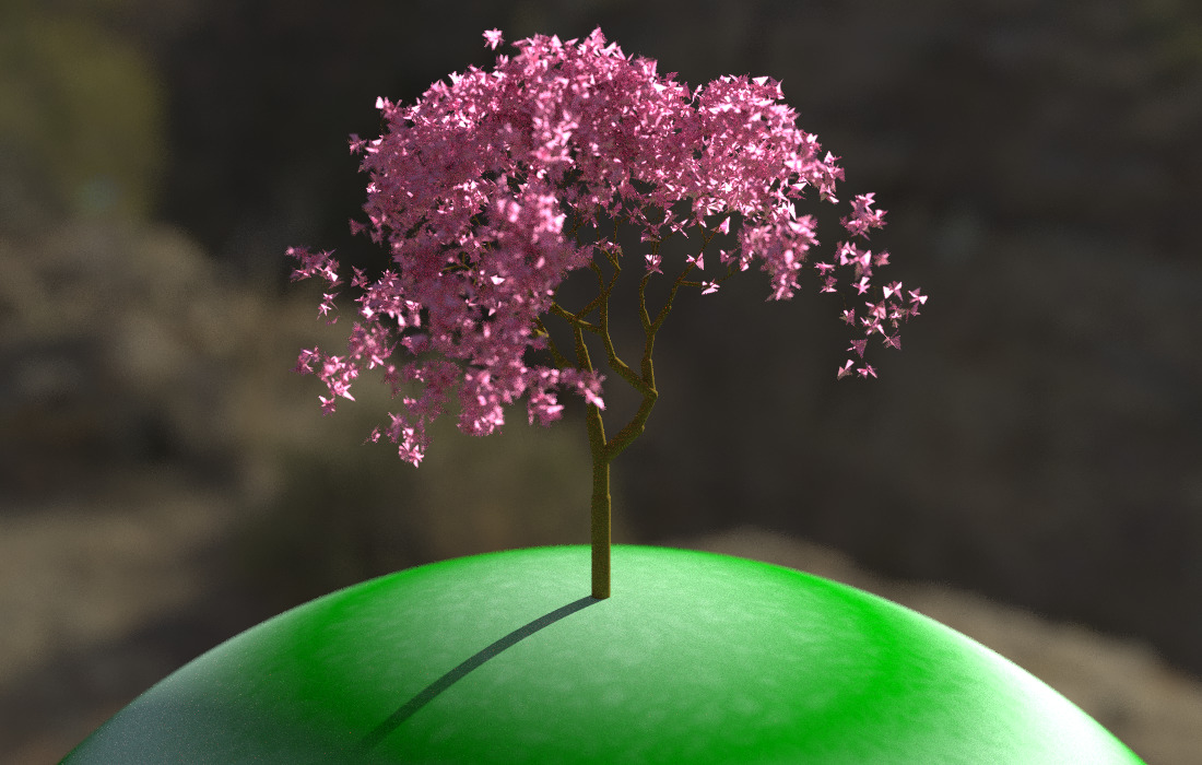
We can also bypass render_tree(), ignore the ground entirely, and just treat the tree like any other rayrender object, placing it anywhere in a scene of our own creation (here we create a nice little bucolic scene in a Cornell box, and render it using rayrender::render_scene()):
tree_pig = generate_tree(seed=121, x=555/2,z=555/2, branch_depth = 9, leaf_color = "chartreuse4",
                         scale = 80, branch_angle_vert = c(-20,0,20), leaf_depth_start = 5)

generate_cornell(lightwidth = 150, lightdepth = 150, lightintensity = 30) %>%
  add_object(tree_pig) %>%
  add_object(group_objects(
    disk(radius=70, inner_radius = 40, z=10, angle = c(90,0,0),
         material = diffuse(color="grey20"),flipped = TRUE) %>%
    add_object(disk(radius=70, inner_radius = 40, z=-10, angle = c(90,0,0),
                    material = diffuse(color="grey20"))) %>%
    add_object(cylinder(radius=70, length=20, angle = c(90,0,0),
                        material = diffuse(color="grey20"))) %>%
    add_object(cylinder(radius=40, length=20, angle = c(90,0,0),
                        material = diffuse(color="grey20"))),
    group_angle = c(0,30,0), group_translate = c(400,110,555/2))) %>%
  add_object(segment(start = c(400,150,555/2), end =  c(400,310,555/2), radius=3)) %>%
  add_object(ellipsoid(x=400, y=165,z=555/2,a=5,b=20,c=20,angle=c(0,50,0))) %>%
  add_object(ellipsoid(x=405, y=165,z=555/2,a=5,b=20,c=20,angle=c(0,50,0))) %>%
  add_object(ellipsoid(x=399, y=165,z=555/2,a=5,b=20,c=20,angle=c(0,50,0))) %>%
  add_object(pig(x=150,z=300,y=85,angle=c(0,50,0),scale = 50, emotion = "skeptical")) %>%
  add_object(ellipsoid(x=555/2,z=555/2,a=200,b=20,c=200,material=diffuse(color="tan"))) %>%
  render_scene(width=1200, height=1200, clamp_value=10, samples=400, sample_method = "stratified")
## Setting default values for Cornell box: lookfrom `c(278,278,-800)` lookat `c(278,278,0)` fov `40` .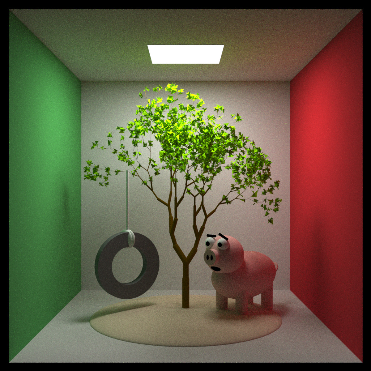
And finally, we can create animations like the one featured at the top by varying the inputs and saving each frame to an image. After all the frames have been rendered, we combine with the {av} package (R ffmpeg wrapper) into a movie:
t_steps = seq(0,360,length.out = 61)[-61]
branch_angle1 = 15 * sinpi(t_steps/180)
branch_angle2 = 10 * sinpi(t_steps/180+30/180)
branch_angle3 = 10 * sinpi(t_steps/180+60/180)


for(i in seq(1,60,by=1)) {
  generate_tree(seed = 2222, branch_angle_vert = c(-20,20) + branch_angle2[i]/2,
                branch_angle = seq(-45,45,by=5),
                branch_depth = 8, leaf_color = "chartreuse4",
                leaf_depth_start = 5, branch_color = "tan") %>%
    add_object(group_objects(generate_tree(seed = 3333,
                             branch_angle_vert = c(-15,15) + branch_angle1[i]/2,
                             branch_depth = 8 , leaf_color = "dodgerblue4",
                             leaf_depth_start = 5, branch_color = "tan"),
               pivot_point = c(0,-10,0),group_angle=c(0,0,-15))) %>%
    add_object(group_objects(generate_tree(seed = 4444,
                             branch_angle_vert = c(-10,10) + branch_angle3[i]/2,
                             branch_depth = 8, leaf_color = "magenta",
                             leaf_depth_start = 5, branch_color = "tan"),
               pivot_point = c(0,-10,0),group_angle=c(0,0,15))) %>%
    raybonsai::render_tree(lights = FALSE, environment_light = "symmetrical_garden_2k.hdr",
                           width=1200, height=800, aperture=0.5,
                           filename = glue::glue("wave{i}"),
                           fov=25,lookfrom=c(0,5,20), lookat=c(0,2,0),
                           rotate_env=-90, sample_method="stratified")
}

av::av_encode_video(glue::glue("wave{1:60}.png"), output = "treewave.mp4", framerate = 30)Now go forth and digitally garden! Check out the package site/Github for more information
Site: www.raybonsai.com
Github: Github Repo
And if you make something cool, feel free to share it on Twitter with the hashtags #rstats and #rayrender so people can see what you’ve planted.