Roadtripping America in R: Turning Spatial Data into Animations with Rayshader
What’s cooler than spinning 3D animations of geospatial data? Flying spinning 3D animations of geospatial data! And that’s what this blog post is going to teach you how to make, using new features in rayshader that make the process simple and straightforward. Normally, I’d also try to give you a little more background about the motivation for making this feature, and why (and when) you should consider using it. But now I have an active one year old and about 30-45 minutes free time each night, so here’s the abridged version:
- There’s lots of data about travel over 3D landscapes, and traveling along the path in 3D can be interesting, e.g. strava run/cycling data, animal GPS tracks, trails and hiking paths
- Spinning makes the visualization more cinematic (more drone footage, less Playstation 1 fixed camera)
- It’s fun (isn’t that way really matters?) and makes even the most boring data interesting and dynamic
And what’s one of the most boring data sets available? The US interstate system! Apologies to all Federal Highway Administration employees reading this blog post. The interstates have (basically) been finished for half a century—there’s nothing new or dynamic about them. But taking a road trip across the country is an American pasttime, so why not do it in R?
Let’s start by loading all the packages we’ll need. We’ll also need to install the developmental version of rayshader from github:
# remotes::install_github("tylermorganwall/rayshader")
library(sf)
library(terra)
library(raster)
library(dplyr)
library(ggplot2)
library(rayshader)
library(rgl)
library(spData)
sf_use_s2(FALSE)
Now we’ll load our data. The elevation data is from GEBCO, which combines topographic with bathymetric data in a single global dataset, which makes for easy plotting. We’ll load it with the {terra} package, using terra::rast(). The highway data is from data.gov (get it here: https://catalog.data.gov/dataset/tiger-line-shapefile-2016-nation-u-s-primary-roads-national-shapefile), which we’ll load with sf::st_read(). We’ll also rename the spData::us_state dataset to mainland_us, purely for convenience.
all_earth = rast("~/Desktop/spatial_data/gebco_2022_sub_ice_topo/GEBCO_2022_sub_ice_topo.nc")
highwaydata = st_read("~/Desktop/spatial_data/tl_2016_us_primaryroads/tl_2016_us_primaryroads.shp")
## Reading layer `tl_2016_us_primaryroads' from data source
## `/Users/tyler/Desktop/spatial_data/tl_2016_us_primaryroads/tl_2016_us_primaryroads.shp'
## using driver `ESRI Shapefile'
## Simple feature collection with 12509 features and 4 fields
## Geometry type: LINESTRING
## Dimension: XY
## Bounding box: xmin: -170.8313 ymin: -14.3129 xmax: -65.64866 ymax: 49.00209
## Geodetic CRS: NAD83water_bodies = st_read("~/Desktop/spatial_data/USA_Detailed_Water_Bodies/USA_Detailed_Water_Bodies.shp")## Reading layer `USA_Detailed_Water_Bodies' from data source
## `/Users/tyler/Desktop/spatial_data/USA_Detailed_Water_Bodies/USA_Detailed_Water_Bodies.shp'
## using driver `ESRI Shapefile'
## Simple feature collection with 463591 features and 7 fields
## Geometry type: MULTIPOLYGON
## Dimension: XY
## Bounding box: xmin: -160.2311 ymin: 19.204 xmax: -66.99787 ymax: 49.38433
## Geodetic CRS: WGS 84mainland_us = spData::us_stateThe highway data includes all interstates in the country: let’s only pull out I-80, which stretches from the San Francisco, CA to Teaneck, NJ (both equally famous cities).
head(highwaydata)## Simple feature collection with 6 features and 4 fields
## Geometry type: LINESTRING
## Dimension: XY
## Bounding box: xmin: -122.6895 ymin: 38.34893 xmax: -75.61068 ymax: 45.54082
## Geodetic CRS: NAD83
## LINEARID FULLNAME RTTYP MTFCC geometry
## 1 1105647111403 Morgan Branch Dr M S1100 LINESTRING (-75.61562 38.62...
## 2 1103662626368 Biddle Pike M S1100 LINESTRING (-84.56702 38.36...
## 3 1103662626717 Cincinnati Pike M S1100 LINESTRING (-84.56805 38.34...
## 4 1105056901124 I- 405 I S1100 LINESTRING (-122.6796 45.54...
## 5 1105056901128 I- 405 I S1100 LINESTRING (-122.671 45.506...
## 6 1105056901162 I- 70 I S1100 LINESTRING (-85.2209 39.853...i80data = highwaydata |>
filter(FULLNAME == "I- 80")
Now let’s use our polygon data to compute a bounding box (using sf::st_bbox()) for the USA, which we’ll then use to crop (using terra::crop()) our global elevation data. We’ll also reduce the resolution by a factor of 8 using terra::aggregate() so our 3D model isn’t gigantic, and create an elevation matrix out of it using rayshader’s raster_to_matrix() function. We’ll also shave off the last and first rows, as for some reason they come back as NA values.
bbox = st_bbox(mainland_us)

just_usa = crop(all_earth, bbox) |>
  aggregate(8)

usa_mat = raster_to_matrix(just_usa)
usa_mat_nan1 = usa_mat[,-ncol(usa_mat)]
usa_mat_nan2 = usa_mat_nan1[-nrow(usa_mat),]
Let’s make sure all the spatial data is in the same coordinate system by using sf::st_transform() and sf::st_crs(). We’ll transform all the other spatial objects to the {terra} object’s coordinate system:
crs_us = mainland_us |>
  st_transform(st_crs(just_usa))

usa_water_bodies = water_bodies |>
  st_transform(st_crs(just_usa))
Now let’s filter out the water bodies to only include the large ones (this is so we don’t have to wait around while we process a bunch of small ponds and lakes that aren’t big enough to appear on our map):
big_water_bodies = usa_water_bodies |>
  filter(FTYPE == "Lake/Pond" & SQMI > 100)
And let’s create a color palette we’ll use for the bathymetry data and generate an overlay to apply to all elevations below sea level. This will help distinguish land from the ocean, as we are working with a dataset with combined topographic/bathymetric data. We’ll generate the land data using the default height_shade() palette, and set the minimum altitude to 0. We’ll then plot this map with plot_map().
water_palette = colorRampPalette(c("darkblue", "dodgerblue", "lightblue"))(200)
bathy_hs = height_shade(usa_mat_nan2, texture = water_palette)

usa_mat_nan2 |>
  height_shade(range = c(0,max(usa_mat_nan2))) |>
  add_overlay(generate_altitude_overlay(bathy_hs, heightmap = usa_mat_nan2,
                                        start_transition = 0, lower = TRUE)) |>
  plot_map()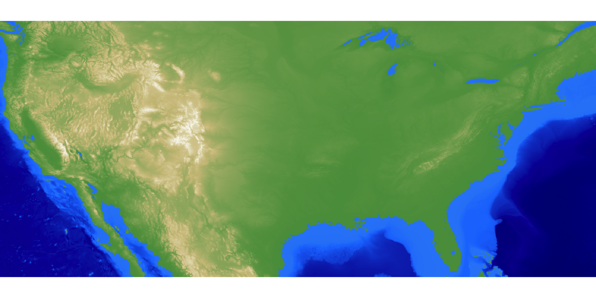
Now let’s render our 3D map! This involves taking our hillshade generated above and adding our overlays for state polygons and large non-oceanic bodies of water in the USA, and then plotting it all in 3D.
usa_mat_nan2 |>
  height_shade(range = c(0,max(usa_mat_nan2))) |>
  add_overlay(generate_altitude_overlay(bathy_hs, heightmap = usa_mat_nan2,
                                        start_transition = 0, lower = TRUE)) |>
  add_overlay(generate_polygon_overlay(big_water_bodies, extent = just_usa, linecolor = NA,
                                       width = nrow(usa_mat_nan2) * 4,height = ncol(usa_mat_nan2) * 4,
                                       heightmap = usa_mat_nan2, palette = "dodgerblue2"),
              rescale_original = TRUE) |>
  add_overlay(generate_polygon_overlay(crs_us, extent = just_usa, linewidth = 16,linecolor ="white",
                                       width = nrow(usa_mat_nan2) * 8,
                                       height = ncol(usa_mat_nan2) * 8, palette = NA),
              rescale_original = TRUE) |>
  plot_3d(usa_mat_nan2,water=FALSE,zscale=200)

render_resize_window(width=1000, height=800)
render_camera(theta = 45, phi = 45, zoom = 0.7)
render_snapshot(software_render = TRUE, fsaa = 2)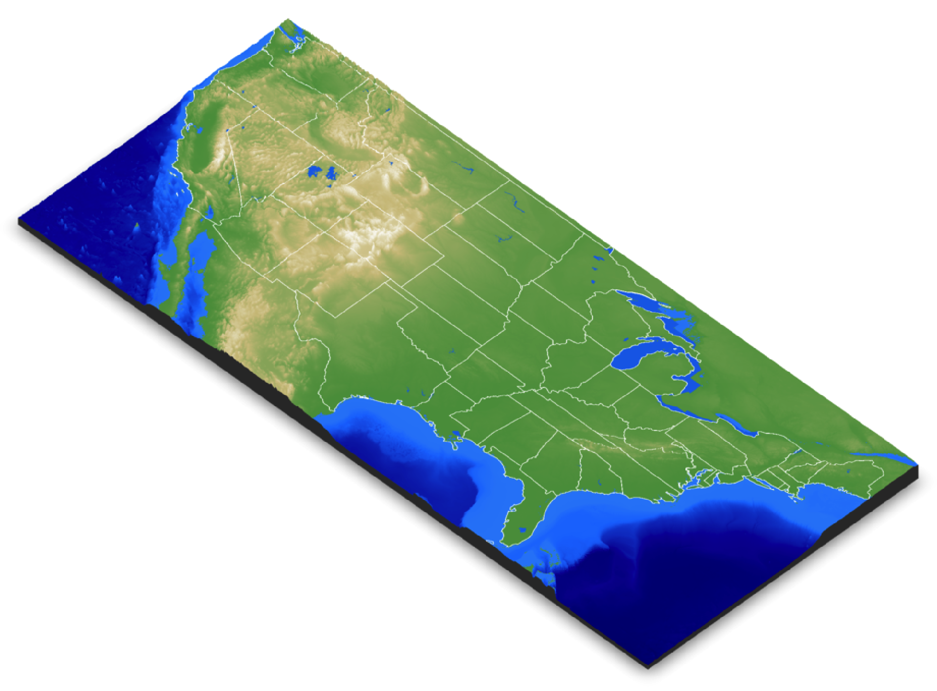
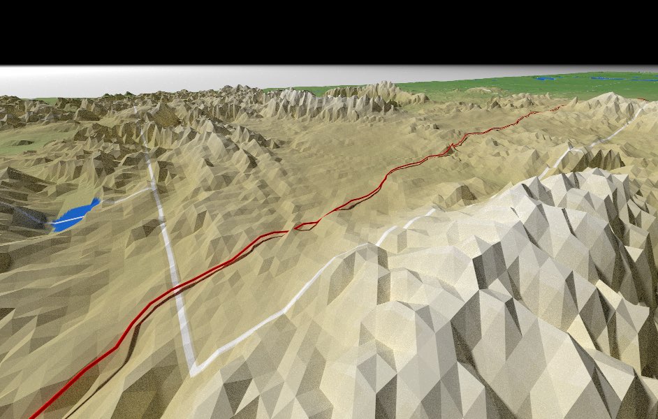
Now we plot our road data using render_path(). We’ll offset this slightly off the ground (using the offset argument) so the actual highway is floating and not half-buried in the ground.
render_path(i80data, extent = just_usa, heightmap = usa_mat_nan2, color="red",
            linewidth = 2, zscale=200, offset = 50)
render_snapshot(software_render = TRUE, fsaa = 2, line_radius = 1)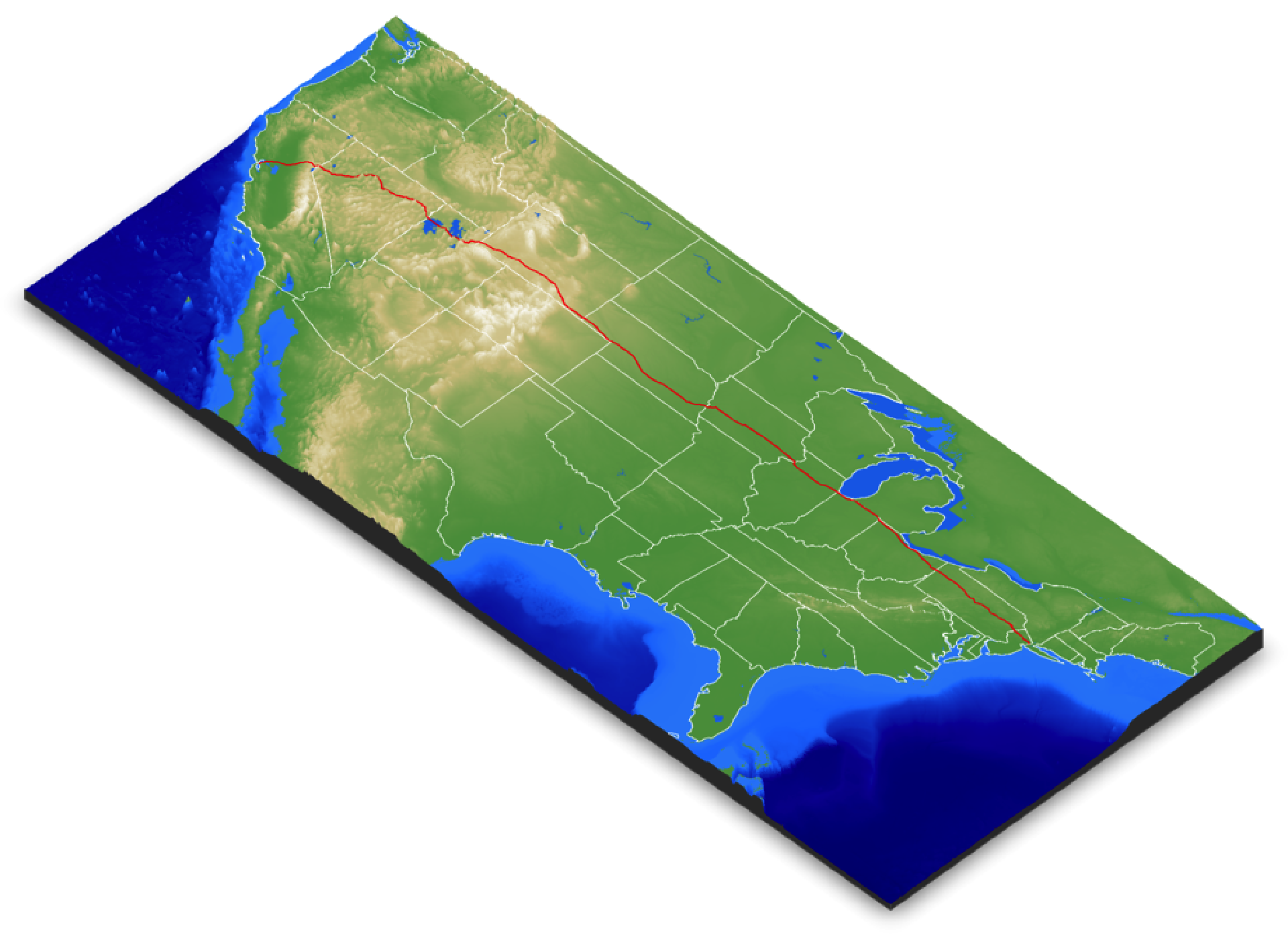
Now to generate our animation: rayshader has a convenient function called convert_path_to_animation_coords() that, unsurprisingly, converts geospatial paths to the coordinate system used by rayshader to create an animation. It takes the path (as defined by a spatial object with “LINESTRING” or “MULTILINESTRING” geometry) and moves the camera at a constant step-size along that path. Here’s where we run into our first problem: if we assume our spatial data is nice and clean and all ready to convert to an animation as-is, we will be sorely disappointed. Let’s visualize what the problem is. The {sf} object here is made up of a series of line objects: let’s plot them in the order they are given in the object. We’ll plot each line segment 1000 units higher than the previous: ideally, the data from rise from one side of the county to the other, indicating the data is arranged sequentially. Is that what we see?
for(i in seq_len(nrow(i80data))) {
  render_path(i80data[i,], extent = just_usa, heightmap = usa_mat_nan2, color="black",
              linewidth = 2, zscale=200, offset = 1000*i)
}
render_camera(theta = 0, phi = 30, zoom = 0.7)
render_resize_window(1200,1000)
render_snapshot(software_render = TRUE, fsaa = 2, line_radius = 1)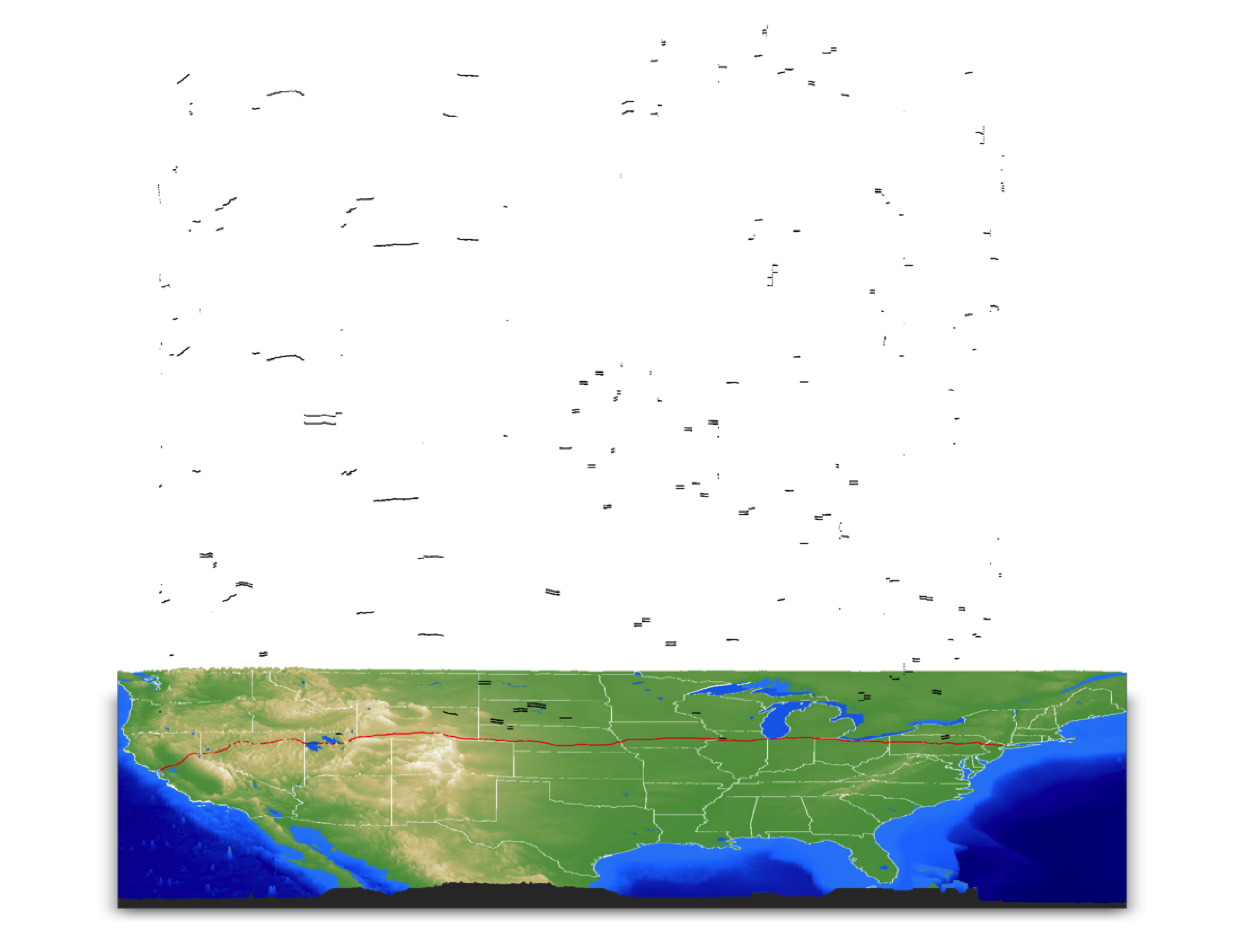
Oh no. Not at all. And even worse, it appears we have duplicates: some (but confusingly, not all!) segments of the highway include both east and west-bound lanes. So we need to remove duplicates and reorder the data so each segment lines up end-to-end. I wrote a nice little helper utility to merge and clean paths in render_path() and convert_path_to_animation_coords() that you can turn on by setting reorder = TRUE. This algorithm first starts by comparing each segment’s end and start points to every other segment’s end and start points (and checking them reversed, in case the line orientation is flipped) and throws away segments where both ends fall within reorder_duplicate_tolerance distance to another segment. It then starts with the segment at row reorder_first_index and then searches for another segment with a start/end point within reorder_merge_tolerance distance and reorders the sf object to make them sequential. Once it can’t find any segments within reorder_merge_tolerance (and if reorder_first_index is greater than 1), it will then do the process in reverse, starting with first segment’s starting point. The algorithm isn’t perfect and needs to be fine-tuned for each dataset with the tolerance values, but as you’ll see: it does the job! (you can also look into sf::st_line_merge() which does something similar, but it didn’t work on this dataset, although it got close).
Let’s now visualize the order of the path segments with reorder = TRUE. We’ll call the internal function that does the reordering so we can show the sequential ordering of the path (represented in the altitude).
i80data_reordered = rayshader:::ray_merge_reorder(i80data,
                                                  merge_tolerance = 0.45,
                                                  duplicate_tolerance = 0.20)

render_path(i80data, extent = just_usa, heightmap = usa_mat_nan2, color="red",
            reorder = TRUE, resample_evenly = TRUE, resample_n = 1000,
            linewidth = 2, zscale=200, offset = 50, clear_previous = TRUE)

for(i in seq_len(nrow(i80data_reordered))) {
  render_path(i80data_reordered[i,], extent = just_usa, heightmap = usa_mat_nan2, color="black",
              linewidth = 2, zscale=200, offset = 1000*i)
}
render_camera(theta = 0, phi = 30, zoom = 0.45)
render_resize_window(1200,600)
render_snapshot(software_render = TRUE, fsaa = 2, line_radius = 1)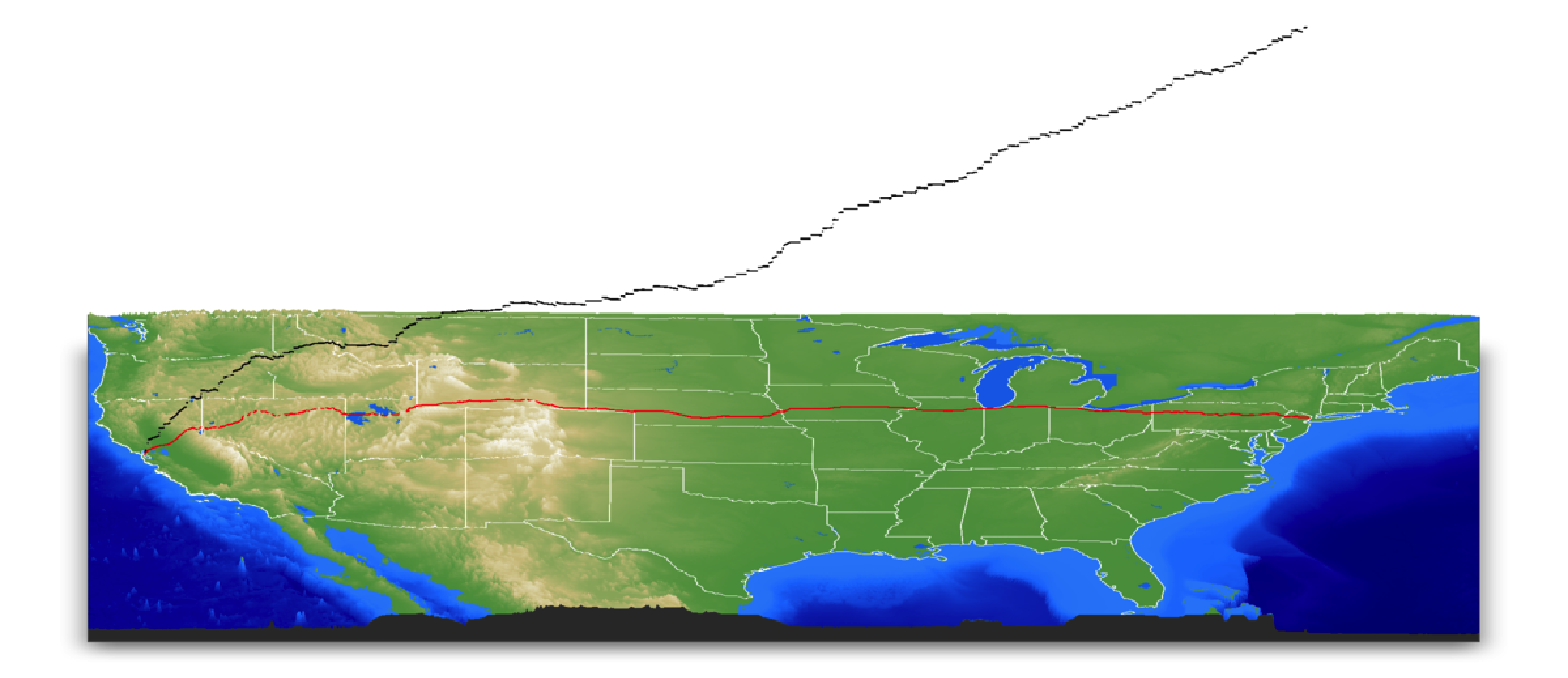
Nice and ordered! Now all the hard work is done. We just need to call convert_path_to_animation_coords() with the proper arguments to get the flyover we want. By default, this function will produce a visualization looking along the path (like a rollercoaster) but I want to make an overhead 3rd person view, so we set follow_camera = TRUE. I’ll also fix the camera’s distance by setting follow_fixed = TRUE and set the offset vector to follow_fixed_offset = c(25,25,25). I’ll damp the motion a bit by setting damp_motion = TRUE and setting damp_magnitude to a value between one and zero. This option smooths the camera motion when it jumps and jerks around too fast.
We can visualize the camera path in black by calling rgl::points3d() in the scene.
camera_coords = convert_path_to_animation_coords(
  i80data,
  extent = just_usa,
  offset_lookat = 1,
  heightmap = usa_mat_nan2,
  zscale = 200,
  offset = 0,
  reorder = TRUE,
  reorder_merge_tolerance = 0.45,
  reorder_duplicate_tolerance = 0.20,
  resample_path_evenly = TRUE,
  frames = 1080,
  follow_camera = TRUE,
  follow_fixed = TRUE,
  follow_fixed_offset = c(25,25,25),
  damp_motion = TRUE,
  damp_magnitude = 0.5
)
render_path(i80data, extent = just_usa, heightmap = usa_mat_nan2, color="red",
            reorder = TRUE,
            linewidth = 2, zscale=200, offset = 50, clear_previous = TRUE)

render_camera(theta = 0, phi = 30, zoom = 0.85)
render_resize_window(1200,1200)
rgl::lines3d(camera_coords[,1:3], color="black", tag = "path3d")
render_snapshot(software_render = TRUE, fsaa = 2, line_radius = 1)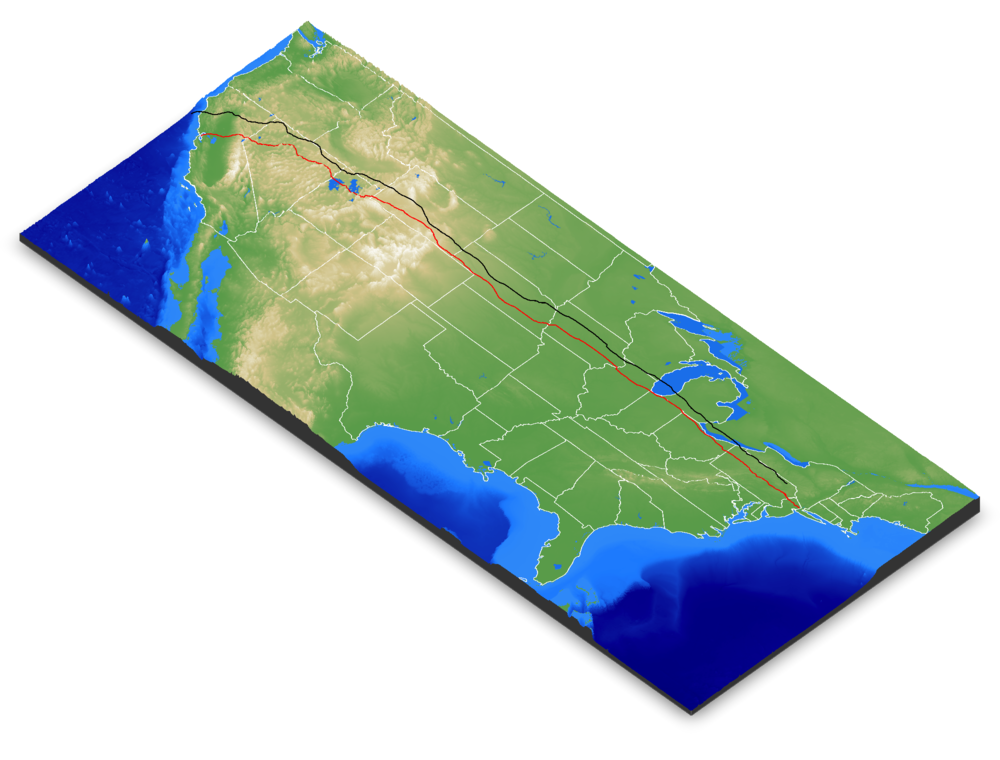
This camera path just directly follows the road. We can use rayshader’s render_highquality(animation_camera_coords = …) interface to pass these coordinates and render all the frames of an animation, and then convert these frames to an video file using ffmpeg (or the {av} package, if you want to work entirely in R).
camera_coords$fov = 80
render_highquality(animation_camera_coords = camera_coords,
                   cache_filename = "cache_america", load_normals = FALSE,
                   samples=128, line_radius=0.10, sample_method = "sobol_blue",
                   filename="roadtrip_frames_fixed")
This animation isn’t bad, but the fixed view is fairly basic and not that interesting. To make the camera view more dynamic and cinematic (following the ideas laid out in this Mapbox blog post), I can tell rayshader to rotate the fixed view around the focal point by setting the follow_rotation argument. I’ll have it execute three full rotations from one side of the county to the other.
Let’s plot the camera motion now to see what that looks like:
rgl::pop3d()
camera_coords = convert_path_to_animation_coords(
  i80data,
  extent = just_usa,
  offset_lookat = 1,
  heightmap = usa_mat_nan2,
  zscale = 200,
  offset = 0,
  reorder = TRUE,
  reorder_merge_tolerance = 0.45,
  reorder_duplicate_tolerance = 0.20,
  resample_path_evenly = TRUE,
  frames = 1080,
  follow_camera = TRUE,
  follow_fixed = TRUE,
  follow_fixed_offset = c(25,25,25),
  follow_rotations = 3,
  damp_motion = TRUE,
  damp_magnitude = 0.5
)
render_camera(theta = 90, phi = 45, zoom = 0.65)
rgl::lines3d(camera_coords[,1:3], color="black", tag = "path3d")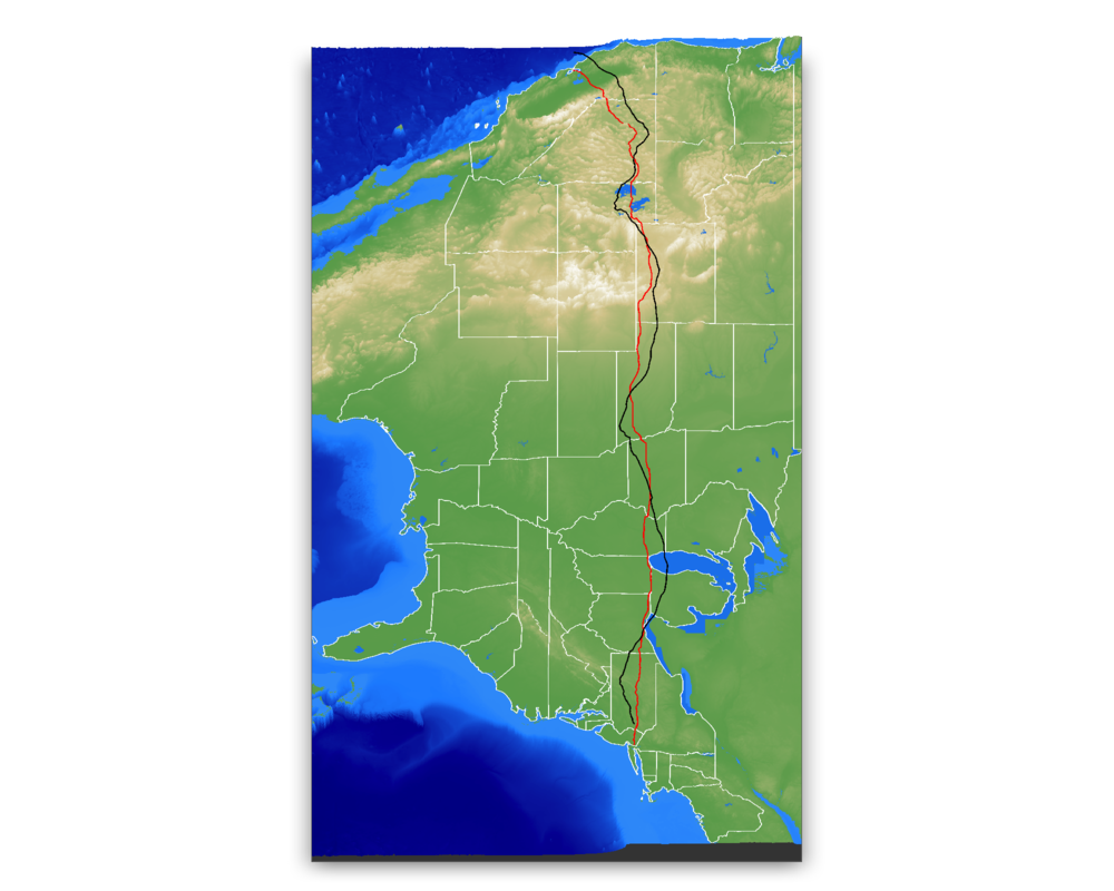
Great! You can see the path orbits around the path, which when combined with the movement along the path results in a cycloid-like movement pattern when viewed from above. Now let’s generate our final, high-quality pathtraced animation. We can pass these coords to animation_camera_coords in render_highquality() to render all the frames for our animation. I’ll also reverse the video to run in the opposite direction, so we end the animation traversing the exciting mountain west rather than the comparatively flat (and boring) northeast. You might think pathtracing 1080 frames would take an outrageously long time (especially since R is “only good at statistics”😉), but by setting the sample method to “sobol_blue”, the adaptive pathtracing in rayrender will speed through the frames fairly quickly (in just a few hours!). In less time than the equivilent cross-country flight, at least :).
render_highquality(animation_camera_coords = camera_coords[nrow(camera_coords):1,], width=800, height=800,
                   samples=128, line_radius=0.10, sample_method = "sobol_blue",
                   filename="roadtrip_frames")
Now we go to the terminal to turn this frames into a movie with ffmpeg. You can also do this with the {av} package in R, but I’m going to be doing something a little more advanced in a second that will require the command line version of ffmpeg.
> ffmpeg -framerate 24 -i roadtrip_frames%d.png -pix_fmt yuv420p roadtrip_frames_better.mp4Now, this final animation is a little fast. We can slow down the video to a reasonable speed by rendering in ffmpeg at half the framerate, from 24 to 12 frames per second.
> ffmpeg -framerate 12 -i roadtrip_frames%d.png -pix_fmt yuv420p roadtrip_frames_slow.mp4You might note that this does make the video unwatchably choppy, but we can pull a little ffmpeg magic out of our hat and fix that without requiring us to do any more expensive pathtracing. Since the camera movement in our animation is fairly smooth, we can actually use motion interpolation to fill in the missing frames. Yes, motion interpolation: the weird soap opera effect that completely ruins the aesthetic of movies at your relative’s house during the holidays. We call ffmpeg with the following script to add motion interpolation to get our smooth road trip across America.
> ffmpeg -i roadtrip_frames_slow.mp4 -filter:v "minterpolate=fps=24:mi_mode=mci:mc_mode=aobmc:me_mode=bidir:vsbmc=1" roadtrip_frames_interpolated.mp4Great! The only downside of motion interpolation here are slight visual artifacts at the edge of the frame, but here it’s not that noticeable most of the time. In just a few lines of code (and a few hours of render time), we’ve created an animation traveling across all of America, entirely in R. You can imagine all the different types of data you might use this for: trips, hikes, animal tracks, bike rides, Twitter CEO flights—the list is endless. Try it on your own data—you might be surprised how you can bring life to an otherwise unassuming spatial dataset by adding a little cinematic 3D magic!