Throwing Shade at the Cartographer Illuminati: Raytracing the Washington Monument in R
When reading older scientific literature, I occasionally run across a statement that never fails to capture my interest. “This method is computationally expensive and should be avoided.” -A statement made around the period Chambawamba captured the zeitgeist of the 90s. These statements are of a particular interest to me in fields where computation is simply a means to an end and not the main focus of researchers–this means that potentially, the issue hasn’t been revisited since it was originally declared algorithm non grata. The last couple decades have delivered us some incredible improvements in CPU power. Algorithms that may once been seen as unworkably greedy may–especially with the help of multiple cores and GPUS–be surprisingly workable. So begins this blog post.
“This method is computationally expensive and should be avoided.” - A statement made around the period Chambawamba captured the zeitgeist of the 90s.
I was reading Twitter when I found a blog post (“How to make a shaded relief in R”, by Elio Campitelli). The post describes how to create the type of shaded relief maps used in cartography programatically in R. Before I read the full article, I read the title and thought: “Cool project! Raytracing topographic maps to simulate light falling on mountains and shade the map appropriately.” After clicking the link and reading about the method used, I was less enthused; the method used was not at all what I thought it would be.
Elio’s original implementation just had a bug that’s long since been fixed–a proper lambertian shading model would look like the example on the right.
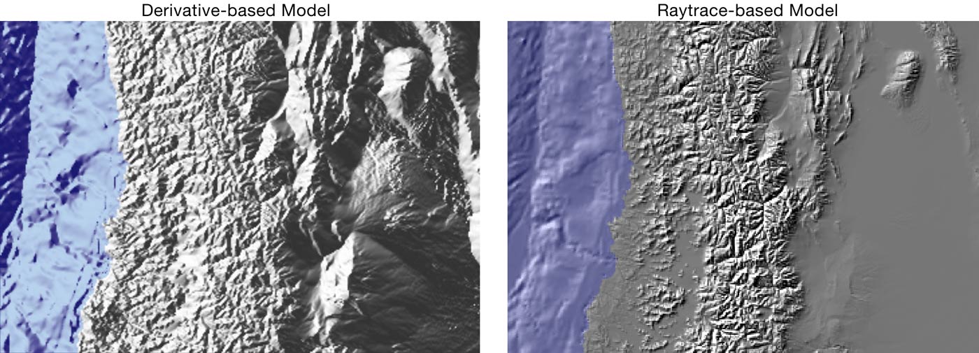
It’s not that I didn’t find what he did interesting–I just had one of those moments where you think you know how something is going to be done and then are sorely disappointed when, well, it wasn’t done that way. His cartographer-tested-and-approved method is calculating the local slope at each point (by taking the gradient of the data) and–depending on the direction of the slope compared to the light direction–shading the surface . Slopes descending towards the light source will be brighter, and slopes descending away from the light source will be darker. This method is much more computationally efficient than raytracing, but it’s disconnected from the underlying physics of what makes real shadows occur: rays of light not hitting a surface due to another surface in the way.
This is one difference between a local and a global illumination model–a local model just looks at the surface to determine shading intensity, while a global model takes into account the surrounding landscape as well. There’s a great source on all of this that Elio links to, reliefshading.com, that says the following about global illumination:
“Global models, such as ray tracing or radiosity are not well suited for cartographic relief shading, since these models are very computation intensive.” - reliefshading.com, throwing shade.
And not a word more is said on the subject. All of the cited resources from this website all focus on these various local illumination models as well, and it seems the field of cartography decided sometime in the mid-90s that raytracing just wasn’t appropriate for shading topographic maps. And mostly because it was computationally intensive.
Everything was computationally intensive in the 90s.
Mashing your computer’s turbo button was an effective placebo, but it was no way to overcome real algorithmic challenges. Since the cool project I expected to see didn’t actually exist–and was being actively suppressed by the most-certainly-real cartographer illuminati–I had to do it myself.
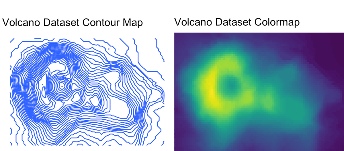
There’s a nice little dataset that comes with R that we’ll be using before moving to actual USGS geographic data: the volcano dataset. It’s a 87x61 heightmap of Maunga Whau Volcano in NZ. Here’s an image of the actual location (thanks Apple maps!), and a contour/heightmap of the data:
> volcano|)
And here’s a gif of the aforementioned cartographer-approved-but-not-what-I-imagined method, with the light source rotating around the image. We rotate the light source around the volcano so you can get a better understanding of how this method shades the slope. It does a pretty good job of representing the topography of the area, and in general, it’s obvious that we’re dealing with some sort of volcano here.
volcano dataset shaded with a derivative-based method.
However, we see one of the pitfalls of this method: the otherworldy fluctuating flat areas in the top right and middle of the image. This is a result of using the derivative to shade the points; when you have a large flat area the color is determined by the boundary (which dictates the derivative), and there will be no variation across the surface. Areas that otherwise look like they should be in darkness–such as the flat steps in the volcano above when the light is coming from the west–appear to be in bright light.
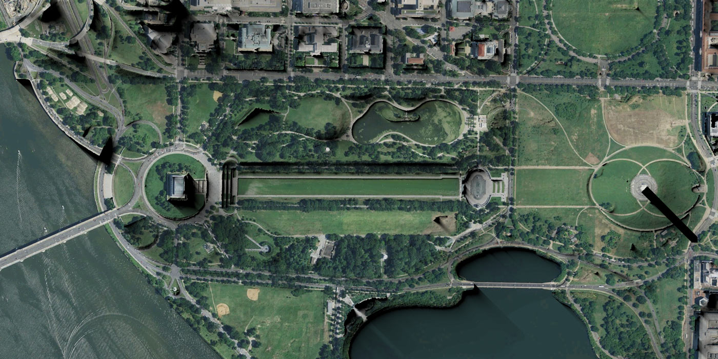
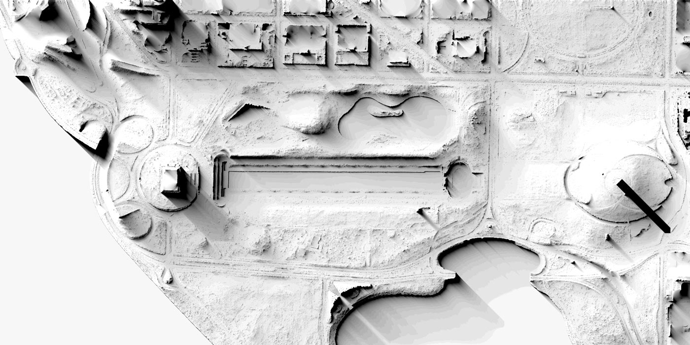
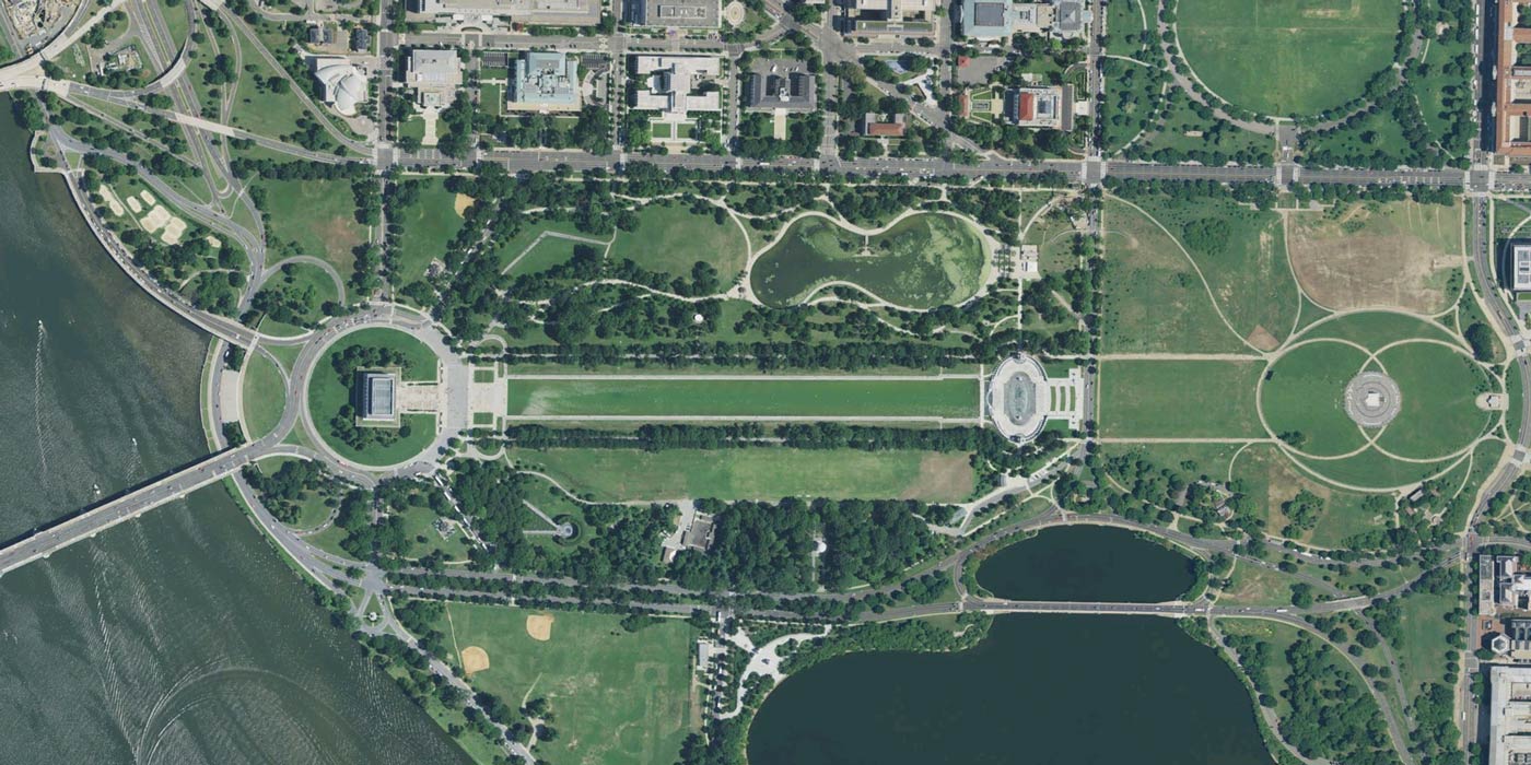
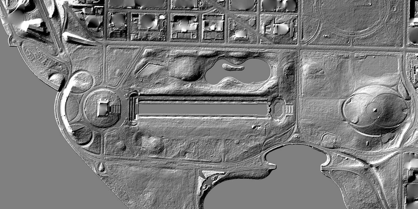
Other than the fluctuating areas, this method seems perfectly fine when trying to image topographic areas. That is, until we look at some more detailed, real data. The fluctuating effect gets even more pronounced when we look at real data with large flat areas, and we run into issues when dealing with irregular man-made objects. Here’s a view of the National Mall in Washington DC through this algorithm:
It’s like someone coated the National Mall with a thin layer of aluminum foil. The reflecting pool’s flat surface creates a fluctuating portal in the center of the image that is 180 degrees out of phase with the water on the edges. Since this real data has lots of low, relatively flat areas with some surface roughness, we also see a lot of “noise” from the small fluctuations in flat areas. Worst of all, there’s no sense of scale–the fact that there’s a large, tall obelisk in the center of the hill to the right is barely noticeable compared to the slight hill it rests on. It’s not that this method isn’t reasonably effective at conveying topology–it’s just not that natural looking.
For natural looking shadows, let’s simulate nature. Let’s build a raytracer.
For natural looking shadows, let’s simulate nature. Let’s build a raytracer.
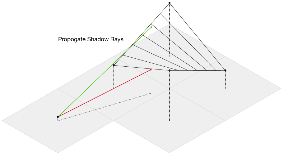
Our data is an evenly spaced square grid of elevation data entered at each point. Our output data will be a grid of light intensities hitting each of those points. We are going to implement what are called “shadow rays”, where we cast a ray in the direction of the light source for a certain distance, and if they intercept a surface, reduce that amount of light at that point. Specifically, we will start with a grid where every point has a value of 1 (indicating full illumination), and cast N rays out at slightly different angles. If the ray intercepts a surface, we will subtract 1/N from that value. If all of the rays intersect a surface, that point on the grid will have an illumination value of 0 (indicating full darkness). By using multiple rays, we will simulate a finite sized light source, which will give us softer shadows than if we only used one ray.
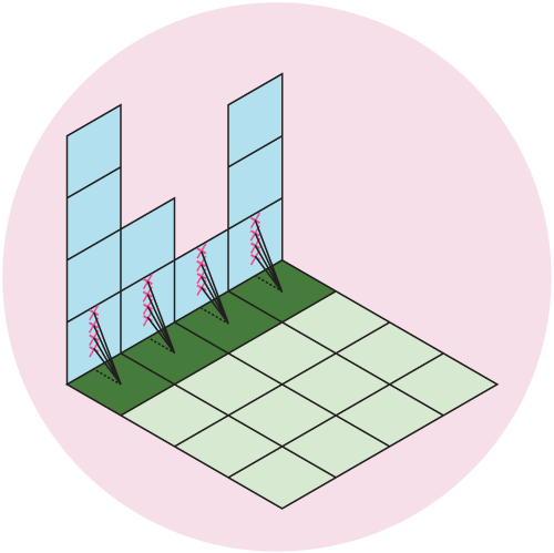
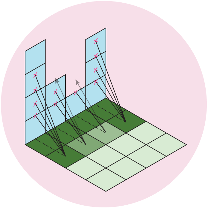
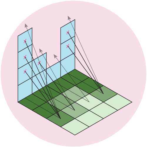
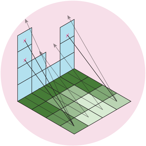
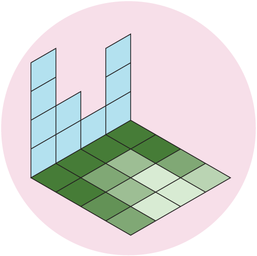
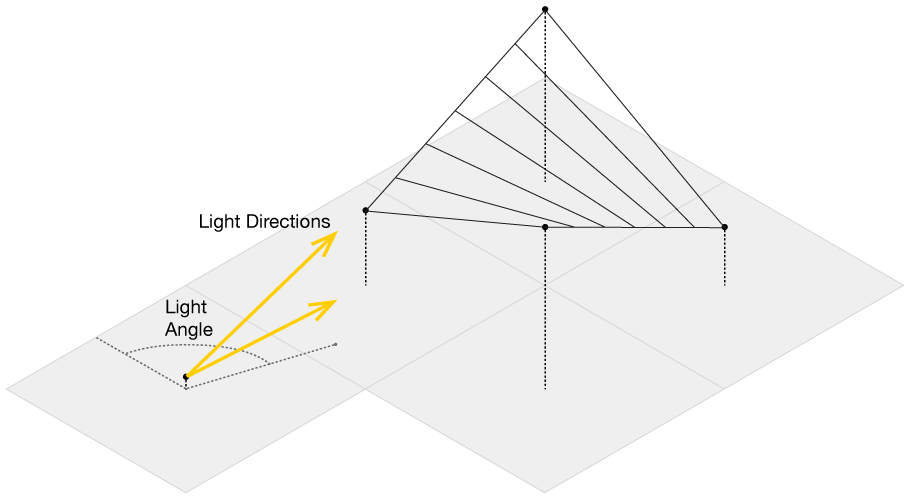
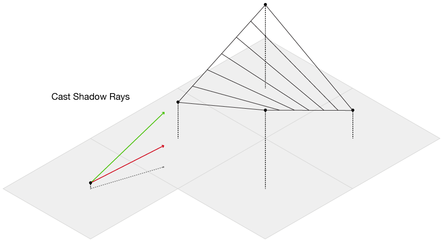
Figure 5: We cast out multiple rays and shade the grid based on the number of intercepted rays. Here, we cast out 4 rays at different angles, which gives us 5 levels of illumination: Full \((I = 1)\), 1/5 rays intercepted \((I = 1-1/5 = 0.8)\), 2/5 rays intercepted \((I = 1-2/5 = 0.6)\), 3/5 rays intercepted \((I = 1-3/5 = 0.4)\), 4/5 rays intercepted \((I = 1-4/5 = 0.2)\), or all rays intercepted \((I = 0)\).
Now, I know there are some technical minded people who started this article thinking: “Cool project! Raytracing topographic maps to simulate light falling on mountains and shade the map appropriately… wait, that’s not a real raytracer.” I look forward to reading your blog post Throwing Shade at the Shade Throwers: Realistically Raytracing the Washington Monument… in Python. But for now, just bear with me–a full complexity raytracer isn’t needed to do what we want to do.
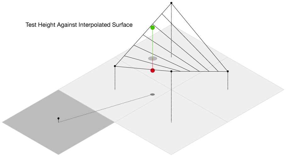
The main complication of this method is our elevation data is defined only at each grid point, while we want to send out rays in more than just the four grid directions. So, we need to be able to check if we are above or below the surface for an arbitrary point on the surface, even between grid points. This immediately presents a challenge from basic geometry–we want to check if we are above or below the surface, but a plane is defined by three points, and on a grid we have four. Thus, linear interpolation doesn’t work, as most of the time there isn’t going to be a single plane that will intercept all four of the points. Thankfully, there is a technique called bilinear interpolation, which allows us to interpolate a surface between four points. We propogate our rays along the grid in the direction of the light source, and then test at each point whether it’s above or below the surface. If it’s below, we immediately stop propogating the ray and subtract one unit of brightness from the origin of the ray.
Luckily, there’s an R function that does bilinear interpolation for us already, so expand the code below to see the basic R implementation.
The original code was not correct (it sampled azimuth angles from -90 to 90, which sort-of combined lambertian shading with raytracing). I’ve updated it to correct for this, but see the ray_shade() function in the rayshader package for a better implementation of this.
library(ggplot2)
library(reshape2)
library(viridis)
volcanoshadow = matrix(1, ncol = ncol(volcano), nrow = nrow(volcano))

volc = list(x=1:nrow(volcano), y=1:ncol(volcano), z=volcano)
sunangle = 45 / 180*pi
angle = 0 / 180 * pi
diffangle = 90 / 180 * pi
numberangles = 25
anglebreaks = seq(angle, diffangle, length.out = numberangles)
maxdistance = floor(sqrt(ncol(volcano)^2 + nrow(volcano)^2))

for (i in 1:nrow(volcano)) {
  for (j in 1:ncol(volcano)) {
    for (anglei in anglebreaks) {
      for (k in 1:maxdistance) {
        xcoord = (i + sin(sunangle)*k)
        ycoord = (j + cos(sunangle)*k)
        if(xcoord > nrow(volcano) ||
           ycoord > ncol(volcano) ||
           xcoord < 0 || ycoord < 0) {
          break
        } else {
          tanangheight = volcano[i, j] + tan(anglei) * k
          if (all(c(volcano[ceiling(xcoord), ceiling(ycoord)],
                    volcano[floor(xcoord), ceiling(ycoord)],
                    volcano[ceiling(xcoord), floor(ycoord)],
                    volcano[floor(xcoord), floor(ycoord)]) < tanangheight)) next
          if (tanangheight < akima::bilinear(volc$x,volc$y,volc$z,x0=xcoord,y0=ycoord)$z) {
            volcanoshadow[i, j] =  volcanoshadow[i, j] - 1 / length(anglebreaks)
            break
          }
        }
      }
    }
  }
}

ggplot() +
  geom_tile(data=melt(volcanoshadow), aes(x=Var1,y=Var2,fill=value)) +
  scale_x_continuous("X coord",expand=c(0,0)) +
  scale_y_continuous("Y coord",expand=c(0,0)) +
  scale_fill_viridis() +
  theme_void() +
  theme(legend.position = "none")
And here is the volcano dataset, shaded by this method. Note there are no odd fluctuating areas like there are with a derivative based method–it looks much more realistic.
volcano dataset shaded with a custom raytracing-based method. Featuring the viridis color palette.
This method works, but it’s un-usably slow for all but small datasets like volcano. I’ve written a R package, rayshader, available at a link at the bottom of the page, that implements a much faster, C++ based version of this algorithm that can quickly shade much larger datasets. It’s much faster than any implementation in R, and has built-in multicore support (that can be activated simply by setting multicore=TRUE) to speed up the rendering process. Many R packages that deal with spatial data require you to convert to a special data format before you can start using them, but all rayshader needs is a base R matrix of elevation points. Feed in the matrix, tell it from what angle(s) the light is coming from, and presto–you’ve got a globally raytraced relief map. Below is some sample code form the rayshader package.
library(rayshader)
library(magrittr)

usgs_data = raster::raster("usgs.img")

#Turn USGS data into a matrix
dc_topographic_map = usgs_data %>%
  extract(.,raster::extent(.),buffer=1000) %>%
  matrix(ncol=10012,nrow=10012)

#Need to add Washington Monument into the data--load heightmap of
#monument and add to topographic map.
washington_monument <- read.csv("washmon.csv", header=FALSE)

lowvals = 3486:3501
highvals = 3519:3534

usgs_data[lowvals,highvals] = usgs_data[lowvals,highvals] +
     as.matrix(washington_monument)

national_mall_map = dc_topographic_map[1700:3700,3000:4000]

sunang = 45*pi/180

angle = 0 / 180 * pi
diffangle = 10 / 180 * pi
numberangles = 30
anglebreaks = seq(angle, diffangle, length.out = numberangles)

single_angle = rayshade(sunangle = sunang,
                        anglebreaks = anglebreaks,
                        heightmap = national_mall_map,
                        zscale = 1,
                        maxsearch = 200,
                        multicore=TRUE)

#image function and ggplot is slow; save with PNG function
#from PNG package.
png::writePNG(t(single_angle), "national_mall_shaded.png")
Applying this function to the same USGS data of the National Mall above, we get this light intensity map:
We can overlay this onto an actual image of the area to get the video at the top of the page (see the code below for the Imagemagick script used to combine the satellite imagery with the shadow map). The raytraced shadows add a much more naturalistic shading to the topography than the local model. The actual length and depth of the shadows can be adjusted by playing with the angles and number of light rays, so this technique can be adapted for many different types of terrain. It also has the additional benefit of playing well with man-made structures; unlike a gradient-based model, this method will more clearly display buildings and extremely sharply changing terrain.

Here’s the bash script using Imagemagick that combines all 144 shadow maps with the satellite image to get the video you see at the top of the page.
#Bash script using Imagemagick to multiply shadow map with background satellite image
for i in {1..144};
  do convert background.png \( washmon_$i.png -normalize +level 0,100% \) -compose multiply -composite washmonmultiply_$i.png;
done
Now, this method does has some downsides that make it less well-suited for actual cartographic work. Firstly, tall objects that cast long shadows will obscure the smaller topolographic features that lie in the shadow. There’s a tradeoff between realism and actual topographic information–real shadows can tell you about the relative height of two objects, but nothing about the slope of the land in the shadow itself. Secondly, it can be difficult to choose a suitable light elevation if the topography of the area has sharp transitions between flat and elevated areas. A low-elevation light (like the sun at dawn or dusk) is better for emphasizing less dramatic topographic features–like the gentle hills and valleys present in the beautiful swampland of DC–but results in very long shadows if a tall object is near. This long aspect ratio increases computation requirements, since one of the arguments is the maximum distance you wish to propagate the ray. Thirdly, cartography has an artistic and practical component, and it’s true what reliefshading.com said in the non-computational shade it threw at global models–sometimes, you need to tweak the direction of the light hitting a particular mountain or valley because it looks better.
And yes, it’s also slower. But computation time is cheap, and CPU cores and GHz are plentiful. To prove my point, here is a 10,012 x 10,012 (100 million point) 10km by 10km (1 meter resolution) map of the DC region, shaded with this method. Each frame took about 30 minutes to compute on my laptop, and consists of five separate light sources to create a nicer gradient.
On the other hand, you can actually adapt this algorithm to produce a local, non-derivative-based shadow map that closely matches the cartographer-approved method, and runs quickly. If you take the maximum propogated distance for each ray down to one unit, you end up sampling how many rays at that point directly intercept the surface. If you send out rays in all directions towards the light–including straight down–the number of rays hitting the surface tells us about the local slope in the direction of the light . You can then use this method to create a locally-shaded model, as seen below.
So, we get the best of both worlds: we can easily produce a local map to show topographic features, or just tweak a few parameters and have a more realistic shadow map that emphasizes tall objects and accurately calculates their shadows. And all of this despite the (ok, mostly imagined) words of a few crusty cartographers. Or, as best put in the immortal words of the baby boomers: Don’t trust any paper over thirty.
Here’s a link to the rayshader github repo with installation and basic usage instructions: