Tutorial: Visualizing Saturn’s Changing Appearance from Earth in R
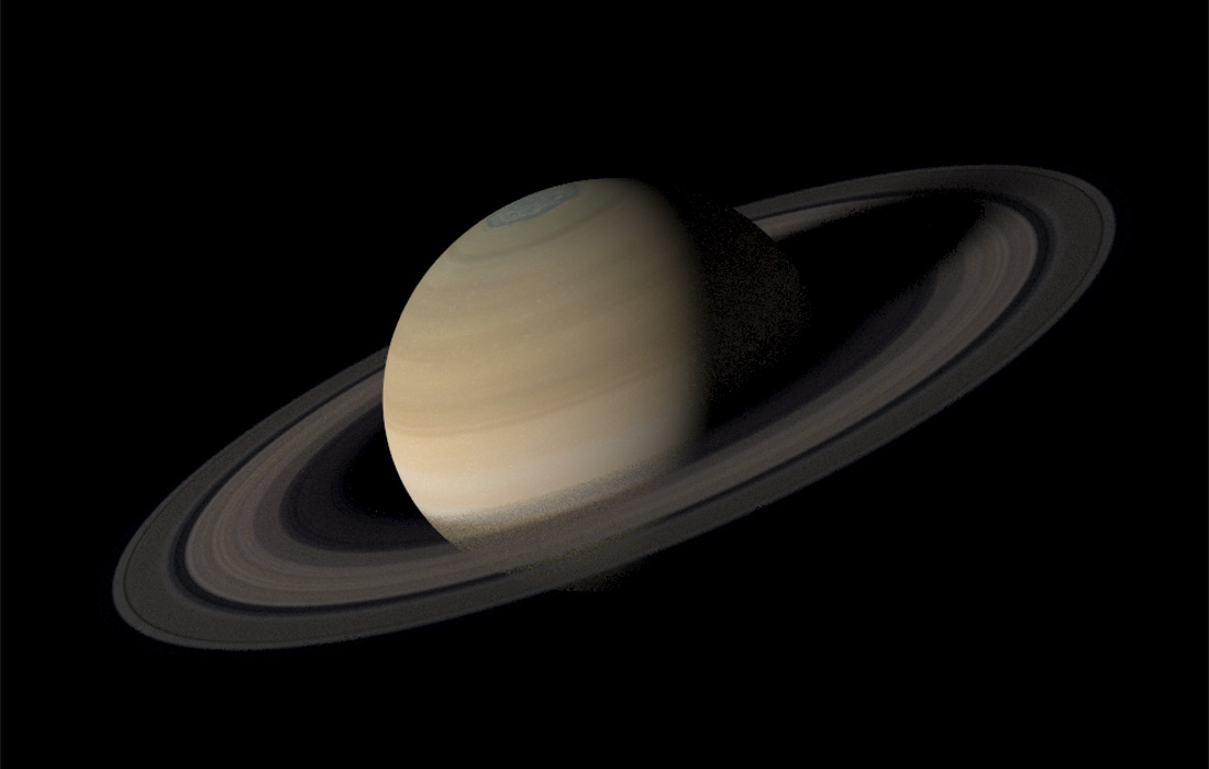
Saturn! The sixth planet from the Sun and the second-largest in the Solar System, named after the Roman god of wealth and agriculture. A planet the universe liked so much it put a ring on it (many rings, in fact). Unlike the rest of the planets, which are just glorified spheres spinning through space, Saturn has a uniquely 3D appearance thanks to its extensive ring system and its 26.7 degree axial tilt. You can have years where the rings are prominently on display when viewed from Earth followed by periods where it almost completely disappears. Question: Can we accurately simulate its appearance from Earth, given a specified date in the future or the past?
Answer: With a little work, yes! Using R and the rayverse, of course. Let me walk you through generating a 3D version of a planet and rendering it from Earth’s perspective, using rayrender (a pathtracer in R).
Generating a 3D planet model itself is relatively simple, as there are many resources for planet textures out there (here’s a link to the Saturn texture from solarsystemscope.com). The planet itself is unique in our solar system due to its extreme oblate-ness: Saturn doesn’t look correct unless you accurately represent its big equatorial bulge (which arises from its rapid 10 hour rotational period). And the ellipsoid object is directly implemented in rayrender, so the planet itself can be represented in a single line of code without any further processing.
ellipsoid(a=0.82,c=0.82,b=0.74, material=diffuse(color="white",image_texture = "2k_saturn.jpg"))) %>%
  group_objects(translate = c(10,0,0), angle=c(26.73,270,0)) %>%
  add_object(sphere(x=0,z=0,y=0,radius=0.125/2,material=light(intensity = 4800*4, invisible = T))) %>%
  render_scene(fov=12,min_variance = 1e-6, clamp_value = 10, lookfrom=c(1,0,0), lookat=c(10,0,0),
               camera_up = c(0,1,0),
               sample_method = "sobol_blue",samples = 256,
width=1000, height=600, aperture = 0) 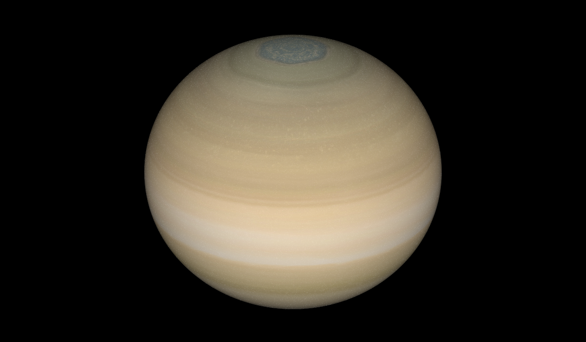
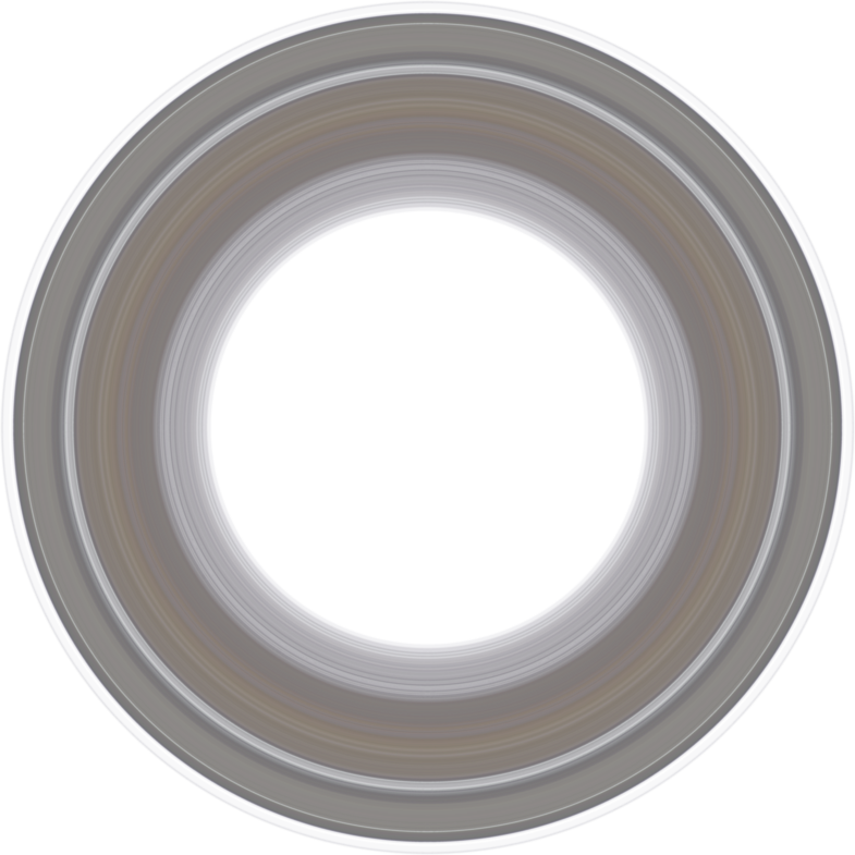
The first real challenge was generating an accurate (size, color, and transparency) representation Saturn’s rings: I needed a texture that I could apply to a flat surface that was centered at Saturn and started and ended exactly where the rings do in space. One google search later, I found the next best thing: a side profile of the ring structure with alpha transparency embedded in the image, with the different ring distances annotated. How to turn this into a full ring texture?

First, let’s load the image into R. We’ll resize it to half its size to ease our memory use when generating the full-sized texture. We’ll also figure out how much padding we need to add to the inner ring based on the start and end of the rings in the texture: the rings start at 66,900 km and end at 139,826 km, and our re-scaled image is 1963 pixels wide. This means the resized image has 37.15 km/pixel, so we need to ensure there are 66,900/37.15 = 1800 pixels of padding in the center of our ring texture before the inner radius of the ring begins.
library(rayrender)
library(lubridate)
##
## Attaching package: 'lubridate'## The following objects are masked from 'package:base':
##
## date, intersect, setdiff, uniolibrary(rayimage)
library(rayvertex)##
## Attaching package: 'rayvertex'## The following object is masked from 'package:rayrender':
##
## r_objfull_ring_slice = png::readPNG("saturn_ring_texture.png")
half_ring_slice = render_resized(full_ring_slice, dims = c(125,3926/2))
inc = (139826-66900)/(3926/2)
padding = 66900/inc
full_width = ncol(half_ring_slice)Now we’ll write a function that calculates a distance based on the image texture pixel to determine what color/opacity the ring should be at that radius. We calculate a radial distance from the center of the image and rescale it based on the padding value we calculated before. We then calculate the weighted value of the two nearest entries in the side-profile texture and return that value.
return_texture = function(i,j,k) {
  distanceval = (sqrt((i-full_width-1)^2 + (j-full_width-1)^2) + 1 ) * (padding + full_width)/full_width

  frac = distanceval - floor(distanceval)
  if(distanceval <= padding+full_width-1 && distanceval > padding+1) {
    half_ring_slice[64,distanceval-padding,k] * (1-frac) +
      half_ring_slice[64,distanceval+1-padding,k] * frac
  } else {
    0
  }
}
We’ll then generate our target image, a 4 layer RGB + alpha array. We then loop through all the pixels in the target image to calculate their color and opacity, and make it 5x smaller to speed up the final render (the lower fidelity won’t matter at the resolution we’re going to render at).
texture_mat = array(0,c(2*(full_width),2*(full_width),4))
for(i in 1:nrow(texture_mat)) {
  for(j in 1:ncol(texture_mat)) {
    texture_mat[i,j,1] = return_texture(i,j,1)
    texture_mat[i,j,2] = return_texture(i,j,2)
    texture_mat[i,j,3] = return_texture(i,j,3)
    texture_mat[i,j,4] = return_texture(i,j,4)
  }
}
texture_mat_small = render_resized(texture_mat,mag=0.2)
Which gives us our texture:
After scaling all the dimensions of the ellipsoid properly, texturing a disk object with the texture we just generated, and rotating it with the proper axial tilt we get a nice accurate representation of Saturn:
disk(radius = 2, inner_radius = 0.9,
     material=diffuse(color="white", sigma = 90,
                      image_texture = texture_mat_small)) %>%
  add_object(ellipsoid(a=0.82,c=0.82,b=0.74,
                       material=diffuse(color="white",
                                        image_texture = "2k_saturn.jpg"))) %>%
  group_objects(angle=c(26.73,11,0), order_rotation = c(1,2,3)) ->
saturn_model

saturn_model %>%
  add_object(sphere(z=12,material=light(intensity = 100))) %>%
  render_scene(fov=18,samples=160,lookfrom=c(10,0,5),width=1000,height=800,
               clamp_value = 10, sample_method = "sobol_blue")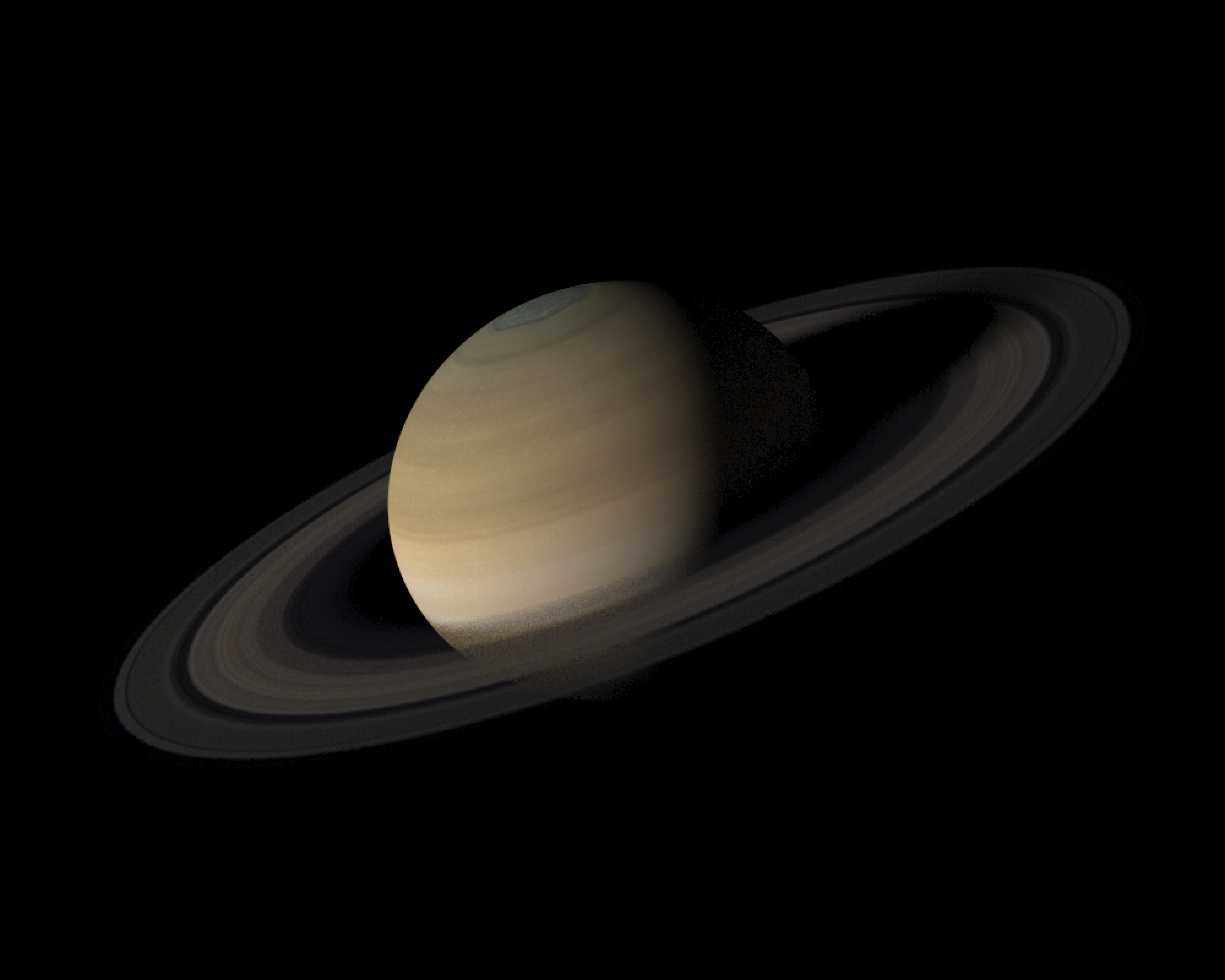
Now: how to render this correctly from the perspective of Earth? That requires calculating the positions of both Earth and Saturn as a function of time. My first instinct was to calculate the positions using Kepler’s laws. There’s a reference coordinate frame (epoch) that starts in the year 2000 (known as J2000) that has reference values that you can use to solve for the approximate positions of the planets (more information available here: https://ssd.jpl.nasa.gov/planets/approx_pos.html#tables). Here’s a function that takes those values and returns the position of the planet (in astronomical units).
earth = list(a  = 1.00000018,
             a_dot = -0.00000003,
             e = 0.01673163,
             e_dot = -0.00003661,
             I = -0.00054346,
             I_dot = -0.01337178,
             L = 100.46691572,
             L_dot = 35999.37306329,
             omega = 102.93005885,
             omega_dot = 0.31795260,
             Omega = -5.11260389,
             Omega_dot = -0.24123856,
             b = 0,
             c = 0,
             s = 0,
             f = 0)

saturn = list(a  = 9.54149883,
             a_dot = -0.00003065,
             e = 0.05550825,
             e_dot = -0.00032044,
             I = 2.49424102,
             I_dot = 0.00451969,
             L = 50.07571329,
             L_dot = 1222.11494724,
             omega = 92.86136063,
             omega_dot = 0.54179478,
             Omega = 113.63998702,
             Omega_dot = -0.25015002,
             b = 0.00025899,
             c = -0.13434469,
             s = 0.87320147,
             f = 38.35125000)


calculate_position = function(date, planet_list) {
  TT = as.numeric(date - ymd("2000-01-01"))/36525
  a0  = planet_list$a
  a_dot = planet_list$a_dot
  e0 = planet_list$e
  e_dot = planet_list$e_dot
  I0 = planet_list$I
  I_dot = planet_list$I_dot
  L0 = planet_list$L
  L_dot = planet_list$L_dot
  peri_long0 = planet_list$omega
  peri_long_dot = planet_list$omega_dot
  Omega0 = planet_list$Omega
  Omega_dot = planet_list$Omega_dot
  b = planet_list$b
  c = planet_list$c
  s = planet_list$s
  f = planet_list$f

  a = a0 + a_dot * TT
  eccentricity = e0 + e_dot * TT
  L = L0 + L_dot * TT
  peri_long = peri_long0 + peri_long_dot * TT
  Omega = Omega0 + Omega_dot * TT
  Ival = I0 + I_dot * TT

  e_star = 180/pi  * eccentricity

  omega = peri_long - Omega
  M = L - peri_long + b * TT^2 + c * cos(f*TT) + s * sin(f * TT)
  while(M < -180) {
    M = M + 360
  }
  while(M > 180) {
    M = M - 360
  }
  tol = 1e-6
  delta_E = 1
  ecc0 = M - e_star * sinpi(M/180)
  eN = ecc0
  #Solve using Newton's method
  while(abs(delta_E) >= tol) {
    delta_M = M - eN - e_star * sinpi(eN/180)
    delta_E = delta_M/(1-eccentricity * cospi(eN/180))
    eN = eN + delta_E
  }
  E = eN
  x_prime = a * (cospi(E/180)-eccentricity)
  y_prime = a * sqrt(1-eccentricity^2) * sinpi(E/180)

  x = (cospi(omega/180)*cospi(Omega/180)  - sinpi(omega/180) * sinpi(Omega/180) * cospi(Ival/180)) * x_prime +
    (-sinpi(omega/180)* cospi(Omega/180) - cospi(omega/180) * sinpi(Omega/180) * cospi(Ival/180)) * y_prime
  y = (cospi(omega/180)*sinpi(Omega/180)  + sinpi(omega/180) * cospi(Omega/180) * cospi(Ival/180)) * x_prime +
    (-sinpi(omega/180)* sinpi(Omega/180) + cospi(omega/180) * cospi(Omega/180) * cospi(Ival/180)) * y_prime
  z = sinpi(omega/180) * sinpi(Ival/180) * x_prime +
    cospi(omega/180) * sinpi(Ival/180) * y_prime
  return(c(x,y,z))
}
I wrote this and rendered the full animation and it appeared to work well initially, but as I looked a little closer things weren’t exactly right. To check if it was correct, I decided to calculate the appearance of Saturn on a few very specific days in the future when the Earth experiences what’s called a ring plane crossing. These are events where the Earth’s viewpoint is exactly aligned with Saturn’s rings, so the rings appear to completely disappear. When I rendered using this method, the ring plane crossings were all a few months off. It turns out this first-order approximate method doesn’t provide enough fidelity to render these events accurately, so I needed to find a better way to get the planet’s positions.
And luckily, I didn’t have to search far! JPL provides a nice, free web interface that you can use to calculate the positions of the planets for a specified range of dates. These positions are much more accurate: It is typically the same data used at JPL for radar astronomy, mission planning, and spacecraft navigation. Selecting Earth and Saturn and exporting daily data from 2020-2050, I generated these datasets:
And loaded them into R using the readr package (with some additional data cleaning steps, which might change depending on the dataset):
library(readr)
horizons_results_earth = read_table2("horizons_results_earth.txt",
                                      col_names = FALSE,
                                     col_types = cols(X9 = col_skip(), X8 = col_skip(),
                                                      X1 = col_skip(), X2 = col_skip(),
                                                      X4 = col_skip(), X10 = col_skip()),
                                     skip = 50)
## Warning: 44 parsing failures.
## row col expected actual file
## 2 -- 10 columns 1 columns 'horizons_results_earth.txt'
## 3 -- 10 columns 1 columns 'horizons_results_earth.txt'
## 18268 -- 10 columns 1 columns 'horizons_results_earth.txt'
## 18269 -- 10 columns 1 columns 'horizons_results_earth.txt'
## 18270 -- 10 columns 1 columns 'horizons_results_earth.txt'
## ..... ... .......... ......... ....................................................
## See problems(...) for more details.horizons_results_earth_t = horizons_results_earth[-(1:3),]
horizons_results_earth_trim = horizons_results_earth_t[-(18265:nrow(horizons_results_earth)),]
colnames(horizons_results_earth_trim) = c("date","x","y","z")
horizons_results_earth_trim$x = as.numeric(gsub(",",x=horizons_results_earth_trim$x,
replacement="",fixed = T))
horizons_results_earth_trim$y = as.numeric(gsub(",",x=horizons_results_earth_trim$y,
replacement="",fixed = T))
horizons_results_earth_trim$z = as.numeric(gsub(",",x=horizons_results_earth_trim$z,
replacement="",fixed = T))
horizons_results_earth_trim$date = ymd(horizons_results_earth_trim$date)
horizons_results_saturn = read_table2("horizons_results_saturn.txt",
col_names = FALSE,
col_types = cols(X9 = col_skip(), X8 = col_skip(),
X1 = col_skip(), X2 = col_skip(),
X4 = col_skip(), X10 = col_skip()),
skip = 47)## Warning: 42 parsing failures.
## row col expected actual file
## 18265 -- 10 columns 1 columns 'horizons_results_saturn.txt'
## 18266 -- 10 columns 1 columns 'horizons_results_saturn.txt'
## 18267 -- 10 columns 1 columns 'horizons_results_saturn.txt'
## 18268 -- 10 columns 1 columns 'horizons_results_saturn.txt'
## 18270 -- 10 columns 9 columns 'horizons_results_saturn.txt'
## ..... ... .......... ......... .....................................................
## See problems(...) for more details.horizons_results_saturn_t = horizons_results_saturn
horizons_results_saturn_trim = horizons_results_saturn_t[-(18262:nrow(horizons_results_saturn)),]
colnames(horizons_results_saturn_trim) = c("date","x","y","z")
horizons_results_saturn_trim$x = as.numeric(gsub(",",x=horizons_results_saturn_trim$x,
replacement="",fixed = T))
horizons_results_saturn_trim$y = as.numeric(gsub(",",x=horizons_results_saturn_trim$y,
replacement="",fixed = T))
horizons_results_saturn_trim$z = as.numeric(gsub(",",x=horizons_results_saturn_trim$z,
replacement="",fixed = T))
horizons_results_saturn_trim$date = ymd(horizons_results_saturn_trim$date)The function to extract planetary positions from this data is much simpler than solving Kepler’s equation: we just index into the data set and extract the desired day (the negative sign is to correct the orientation of the data in our coordinate system).
calculate_saturn_position = function(date) {
  val = as.numeric(horizons_results_saturn_trim[horizons_results_saturn_trim$date == date,c(2,4,3)])
  val * c(-1,1,1)
}

calculate_earth_position = function(date) {
  val = as.numeric(horizons_results_earth_trim[horizons_results_earth_trim$date == date,c(2,4,3)])
  val * c(-1,1,1)
}
Now we use the lubridate package to loop through each week from 2020 through 2050 and render the 3D scene from Earth’s viewpoint (specified via the lookfrom argument in render_scene()). I set the sun as the only light source at the origin, and make it invisible so we can see how Saturn appears without worrying about the Sun occluding our render every other second. We then use ffmpeg to turn these frames into a video.
temp = ymd("2020-Jan-01")
end_date = ymd("2050-Jan-01")
counter = 1

while(temp < end_date) {
  saturn_pos = calculate_saturn_position(temp)
  earth_pos = calculate_earth_position(temp)

  saturn_model %>%
    group_objects(translate = saturn_pos) %>%
    add_object(sphere(x=0,z=0,y=0,radius=0.125,
                      material=light(intensity = 4800, invisible = T))) %>%
    render_scene(fov=25,min_variance = 1e-6, clamp_value = 10,
                 lookfrom=earth_pos, lookat=saturn_pos,
                 sample_method = "sobol_blue",samples = 256, width=1000, height=1000,
                 filename=sprintf("saturn_earth_%d.png",counter),
                 verbose = T,
                 aperture = 0)
  counter = counter + 1
  temp = temp + period("1 week")
}

system("ffmpeg -framerate 24 -i saturn_earth_%d.png -pix_fmt yuv420p saturn.mp4")
I also want to generate a diagram of the solar system showing an overview of Earth and Saturn’s locations (which better shows when they’re in opposition). I do that using the rayvertex package, which is a useful tool for producing more diagrammatic 2D/3D visualizations. I first generate a series of line segments that show the orbits through a full 30/1 year period for Saturn/Earth (respectively):
#Generate Solar System diagram with rayvertex
temp = lubridate::ymd("2000 Jan 01")
end = lubridate::ymd("2030 Jan 01")

saturn_positions = list()
counter = 1
while(temp < end) {
  saturn_positions[[counter]] = calculate_saturn_position(temp)
  temp = temp + period("1 month")
  counter = counter + 1
}

temp = lubridate::ymd("2000 Jan 01")
end = lubridate::ymd("2001 Jan 02")

earth_positions = list()
counter = 1
while(temp < end) {
  earth_positions[[counter]] = calculate_earth_position(temp)
  temp = temp + period("1 week")
  counter = counter + 1
}

scene = segment_mesh(start=saturn_positions[[1]],
                     end=saturn_positions[[2]],radius = 0.1,
                     material = material_list(ambient=c(1,1,1),
                                              diffuse_intensity = 0))

for(i in 2:(length(saturn_positions)-1)) {
  scene = add_shape(scene, segment_mesh(start=saturn_positions[[i]],
                                        end=saturn_positions[[i+1]],
                                        radius = 0.1,
                           material = material_list(ambient=c(1,1,1),
                                                    diffuse_intensity = 0)))
}

for(i in 1:(length(earth_positions)-1)) {
  scene = add_shape(scene, segment_mesh(start=earth_positions[[i]],
                                        end=earth_positions[[i+1]],
                                        radius = 0.1,
                                        material = material_list(ambient=c(1,1,1),
                                                                 diffuse_intensity = 0)))
}
I then add the sun and the planets, and render a cone representing the camera viewpoint from Earth to Saturn. I look through all the days I created views for in the main rendering.
scene = add_shape(scene,sphere_mesh(radius=0.3,
                                    material = material_list(ambient=c(1,1,1),
                                                             diffuse_intensity = 0)))

rasterize_scene(scene, lookfrom=c(0,20,0), lookat=c(0,0,0),camera_up = c(0,0,1),
                fov = 0, ortho_dimensions = c(22,22),
                width=200,height=200, fsaa=4)

temp = ymd("2020-Jan-01")
end_date = ymd("2050-Jan-01")
counter = 1

while(temp < end_date) {
  saturn_pos = calculate_saturn_position(temp)
  earth_pos = calculate_earth_position(temp)

  dir = (saturn_pos - earth_pos)
  dir = dir/sqrt(sum(dir*dir))
  scene %>%
    add_shape(sphere_mesh(radius = 0.45,position=c(0,2,0),
                          material=material_list(ambient="white",
                                                 diffuse="black", dissolve = 1))) %>%
    add_shape(sphere_mesh(radius = 0.4,position=earth_pos + c(0,8,0),
                          material=material_list(ambient="#53a0da",diffuse="black" ))) %>%
    add_shape(sphere_mesh(radius = 0.6,position=saturn_pos+c(0,8,0),
                          material=material_list(ambient="black",diffuse="black" ))) %>%
    add_shape(sphere_mesh(radius = 0.4,position=saturn_pos+c(0,9,0),
                          material=material_list(ambient="white",diffuse="black" ))) %>%
    add_shape(sphere_mesh(radius = 0.8,position=saturn_pos+c(0,7,0),
                          material=material_list(ambient="white",diffuse="black" ))) %>%
    add_shape(cone_mesh(end = earth_pos + c(0,4,0), start = earth_pos + 22 * dir + c(0,4,0), radius=3, material = material_list(ambient="purple", diffuse_intensity = 0,type= "toon",
                         toon_levels = 10, toon_outline_color = "white",
                         toon_outline_width = 0.8))) %>%
    rasterize_scene(lookfrom=c(0,20,0), lookat=c(0,0,0),camera_up = c(0,0,1), fov = 0, ortho_dimensions = c(22,22),
                    width=200,height=200, fsaa=4,
                    filename = sprintf("saturn_diagram%d.png",counter))
  counter = counter + 1
  temp = temp + period("1 week")
}

system("ffmpeg -framerate 24 -i saturn_diagram%d.png -pix_fmt yuv420p saturn_diagram.mp4")I also render a series of images that label each date (using the rayimage package), and turn that into a movie as well.
temp = ymd("2020-Jan-01")
end_date = ymd("2050-Jan-01")
counter = 1
while(temp < end_date) {
  date_title = format(temp, "%b %Y")
  add_title(matrix(0,ncol = nchar(date_title)*40, nrow=60*1.2),
                      title_size  = 60,
                      title_offset = c(10,0),title_text = date_title,
                      title_color = "white",
                      title_position = "east",
                      filename = sprintf("saturn_date%d.png",counter))
  temp = temp + duration("1 week")
  counter = counter + 1
}

system("ffmpeg -framerate 24 -i saturn_date%d.png -pix_fmt yuv420p saturn_dates.mp4")Finally, I also want to include the data on ring crossings, which I got from this website. I used ggplot2 to generate a nice visualization and series of frames to accompany the rendering.
#ring crossings
crossings = c(dmy("23 March 2025"),
              dmy("15 October 2038"),
              dmy("1 April 2039"),
              dmy("9 July 2039"))
crossing_df = data.frame(dates=crossings)

library(ggplot2)
library(ggfx)
library(extrafont)

font_import(paths = "/System/Library/Fonts/",prompt = F)

temp = ymd("2020-Jan-01")
end_date = ymd("2050-Jan-01")
counter = 1

while(temp < end_date) {
  rpc = ggplot() +
    with_bloom(geom_vline(xintercept = crossing_df$dates,color="#22ff22",lwd=0.6),
               threshold_lower=10,strength = 30, sigma = 5)+
    with_bloom(geom_vline(xintercept = temp,color="#ff2222", lwd=0.6 ),
               threshold_lower=10,strength = 30, sigma = 5)+
    scale_x_date("Year",
                 limits=c(ymd("2020-01-01"),ymd("2050-01-01")),
                 date_breaks="2 years", date_labels = "%Y",
                 date_minor_breaks = "1 year") +
    theme_void() +
    labs(title = "    2020-2050 Ring Plane Crossings") +
    theme(panel.background = element_rect(fill="black"),
          plot.background = element_rect(fill="black"),
          panel.grid.major = element_line(color="grey40"),
          panel.grid.minor = element_line(color="grey30"),
          axis.text.y = element_blank(),
          panel.grid.major.y = element_blank(),
          panel.grid.minor.y = element_blank(),
          plot.title = element_text(color="white", size=15,margin=margin(0,0,5,0),
                                    family = "Avenir", face="plain"),
          axis.text = element_text(color="white", size=10, margin=margin(10,0,0,0),
                                   family = "Avenir"),
          plot.margin = margin(10,-10,10,-10, "pt"),
          text = element_text(color="white"))
  ggsave(sprintf("ringplane%d.png",counter),plot=rpc, dpi=100, width=7.6, height=1.8)
  counter = counter + 1
  temp = temp + period("1 week")
}

system("ffmpeg -framerate 24 -i ringplane%d.png -pix_fmt yuv420p ring_plane_plot.mp4")Including this information is useful in two ways: first, ring crossings are the most dramatic change in Saturn’s appearance from Earth over any several-decade long period. If there’s a useful point to this visualization, it’s to know when these events occur. Secondly, from a “data viz engagement” point-of-view, this plot provides the viewer with actual “events” to drive them to continue watching the visualization. The red line moving provides an indication of progress and the green lines indicate that there’s something to look forward to. Otherwise, a viewer might click out after a few seconds of Saturn wobbling over and over again, thinking there’s nothing more to the story.
To complete the visualization, we use ffmpeg to combine all these animations together and add some text:
ffmpeg -i saturn.mp4 -vf "drawbox=x=789:y=789:w=210:h=210:[email protected]:t=fill"  saturn_box.mp4

ffmpeg -i saturn_box.mp4 -i saturn_diagram.mp4 -filter_complex "[0][1]overlay=W-204.5:H-204.5" combined_saturn.mp4

ffmpeg -i combined_saturn.mp4 -y -vf drawtext="fontfile=/System/Library/Fonts/Avenir.ttc: text='View of Saturn from Earth, 2020-2050': fontcolor=white: fontsize=32: box=1: boxcolor=black@0: boxborderw=10: x=20: y=20" -codec:a copy combined_saturn_title.mp4

ffmpeg -i combined_saturn_title.mp4 -y -vf drawtext="fontfile=/System/Library/Fonts/Avenir.ttc: text='Solar System View': fontcolor=white: fontsize=22: box=1: boxcolor=black@0: boxborderw=0: x=805: y=765" -codec:a copy combined_saturn_title_diagram.mp4

ffmpeg -i combined_saturn_title_diagram.mp4 -vf drawtext="fontfile=/System/Library/Fonts/Avenir.ttc: text='Created with rayrender (www.rayrender.net)': fontcolor=white: fontsize=24: box=1: boxcolor=black@0: boxborderw=10: x=20: y=960" -codec:a copy combined_saturn_title_diagram_rr.mp4

ffmpeg -i combined_saturn_title_diagram_rr.mp4 -vf drawtext="fontfile='/System/Library/Fonts/Avenir.ttc: text='Twitter \@tylermorganwall': fontcolor='white': fontsize=24: box=1: boxcolor=black@0: boxborderw=10: x=20: y=930" -codec:a copy combined_saturn_title_diagram_rr_twit.mp4

ffmpeg -i combined_saturn_title_diagram_rr_twit.mp4 -y -vf drawtext="fontfile=/System/Library/Fonts/Avenir.ttc: text='From orbital plane, without sun occlusion': fontcolor='#aaaaaa': fontsize=24: box=1: boxcolor=black@0: boxborderw=10: x=20: y=57" -codec:a copy combined_saturn_title_diagram_rr_twit_for_pedants.mp4

ffmpeg -i combined_saturn_title_diagram_rr_twit_for_pedants.mp4 -i saturn_dates.mp4 -filter_complex "[0][1]overlay=W-325:15" final_saturn.mp4

ffmpeg -i final_saturn.mp4 -i ring_plane_plot.mp4 -filter_complex "[0][1]overlay=20:H-200" final_saturn_for_real_final.mp4
And that’s it! I hope you enjoyed this deep-dive into rendering planets from Earth’s perspective. Feel free to render other astronomical objects using this code, and be sure to post about it using the #rayrender and #RStats hashtags.